Optical convolution¶

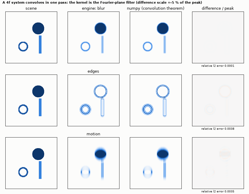
The same 4f layout as a convolution engine. The Fourier-plane filter is the kernel's transfer function; three of them are tried on a scene of a disc, a bar and a ring: a Gaussian blur, edge detection (Laplacian of a Gaussian, signed) and a one-dimensional motion blur (a box along x). The output intensity is compared with numpy's FFT, multiply, inverse FFT.

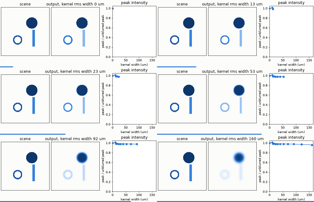
The animation widens the Gaussian kernel from 0 to 160 µm (rms): the filter in the Fourier plane narrows and the image blurs.

python convolution.py

grid 256 x 256, pitch 20 um, f = N dx^2 / lambda = 128.0 mm; the output is intensity |scene * kernel|^2
engine against numpy (FFT, multiply by H, inverse FFT); the errors are printed as bounds, their last digits depend on the FFT library:
blur     correlation above 0.999, relative l2 error below 0.0002
edges    correlation above 0.999, relative l2 error below 0.005
motion   correlation above 0.999, relative l2 error below 0.005
each kernel has N x N taps: N^4 = 4.29e+09 multiply-accumulates for a direct digital convolution, done in one pass of light (4 f / c = 1.71 ns)
worst relative l2 error below 0.005 (the mask and the lens phase are sampled on the grid)
checks passed

What it shows. The convolution theorem holds for the engine's propagation: smooth filters agree to about 10⁻⁴, filters with detail to about 4 x 10⁻³ (the printed values are bounds: 2 x 10⁻⁴ and 5 x 10⁻³). The edge detector is signed in amplitude; the camera sees its square (intensity), as a real sensor would.

Cost. Each kernel has N x N taps, so a direct digital convolution is N⁴ = 4.3 x 10⁹ multiply-accumulates; the optics does it in one transit of 1.7 ns. The engine simulates that on a digital machine in a fraction of a second, with FFTs.