Gallery¶

Figures and animations made by the examples. Generated by python build/gallery.py from the hero.png and animation.gif files next to the example READMEs; python docs/examples/make_all.py redraws them. Each animation is at most 2.5 MB, each figure at most 300 kB.

GettingStarted¶

04 -- Your own n(t, I) in Python¶

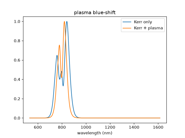
custom_response.py adds a toy plasma (free-carrier) response with memory, and the multiphoton absorption that creates it, to the built-in Kerr effect of a fused-silica plate -- the kind of model the engine cannot know about, supplied as a vectorised NumPy function:

18 -- A nonlinear medium you define: n(x, y, z, t, I, F)¶

A 10 mm "doped glass" rod on a radial grid.

00 -- Python quick start¶

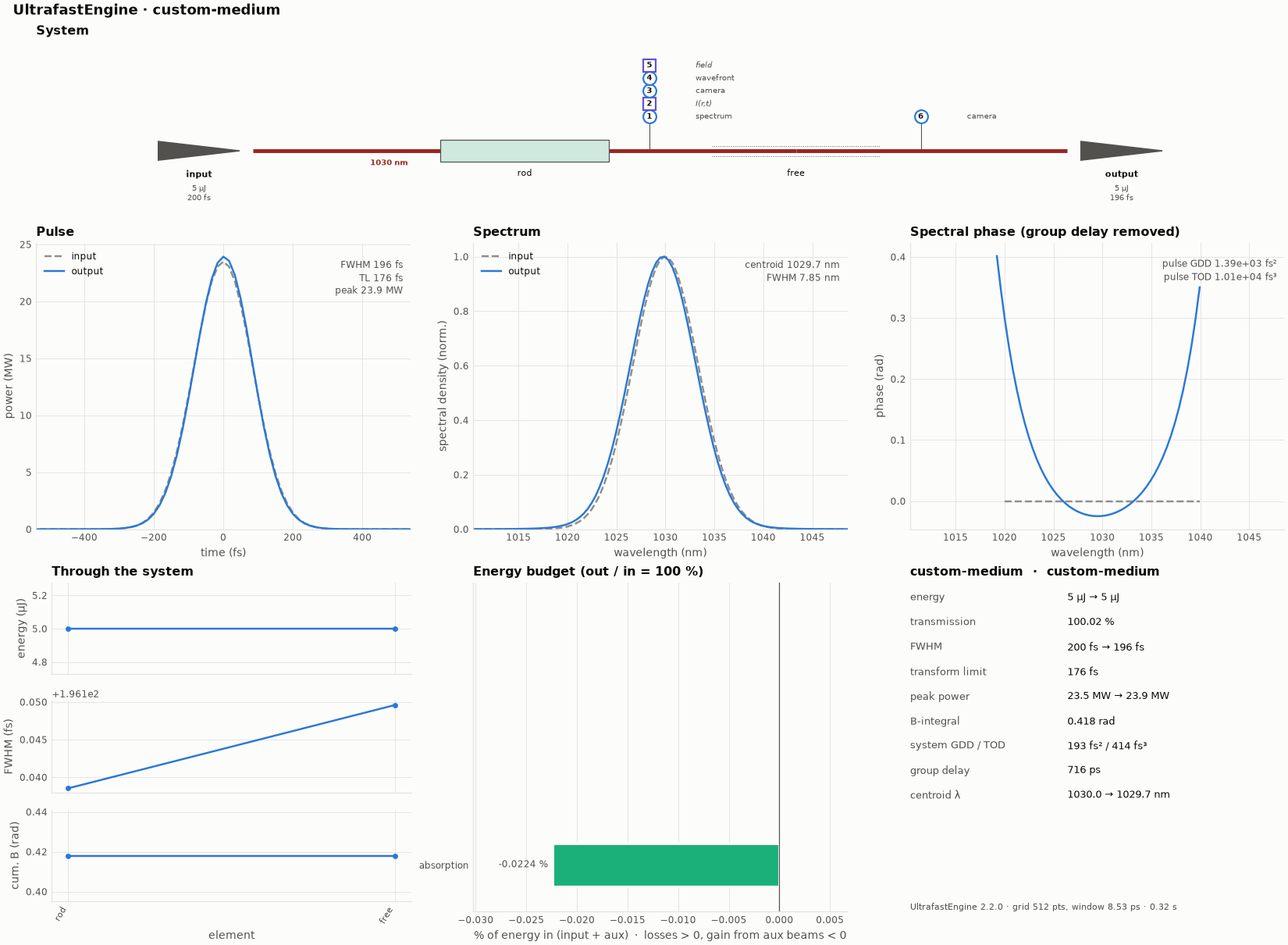
Build a system in Python, run it, read the results and scan a parameter.

LaserSystems¶

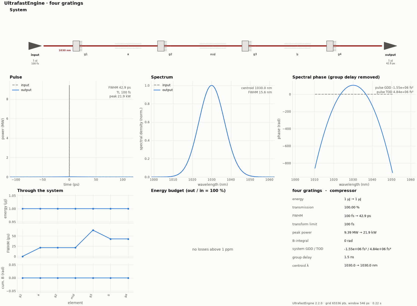
38 -- A four-grating compressor, grating by grating¶

A compressor on the command line.

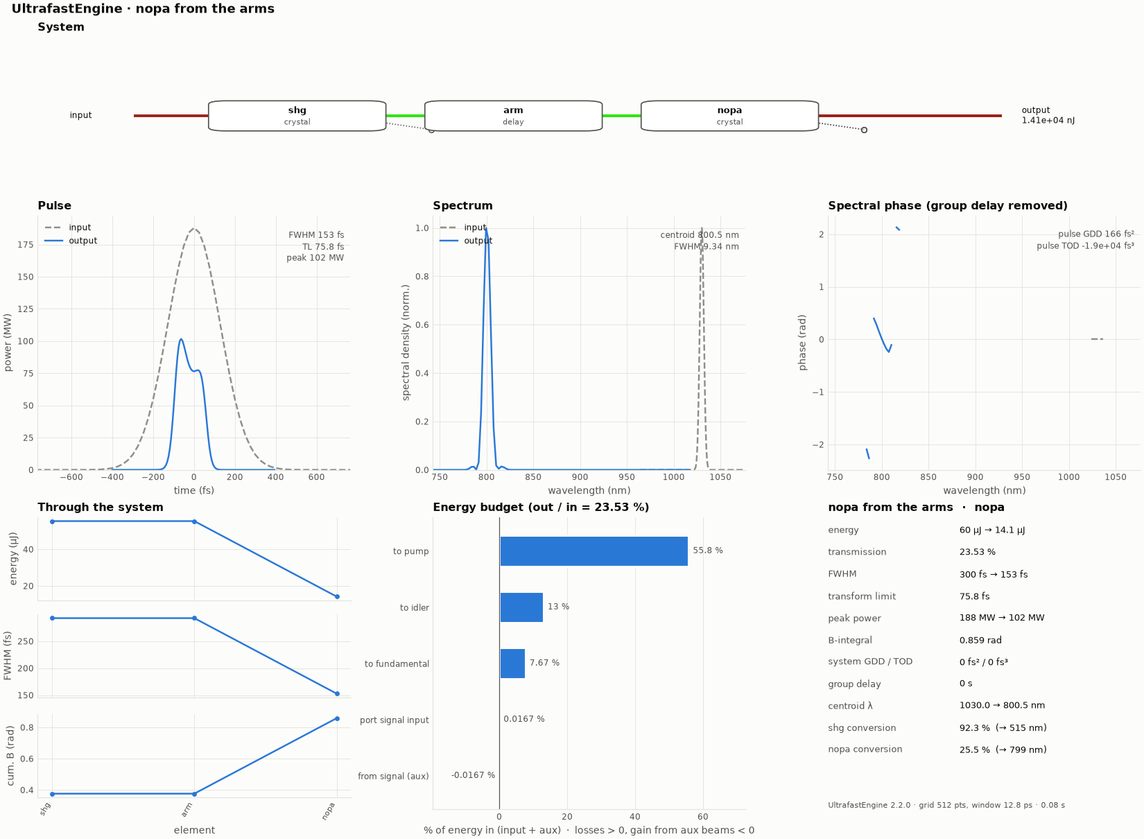
42 -- A non-collinear OPA with the angle from the pump arm¶

A NOPA on the command line, as a Branched system.

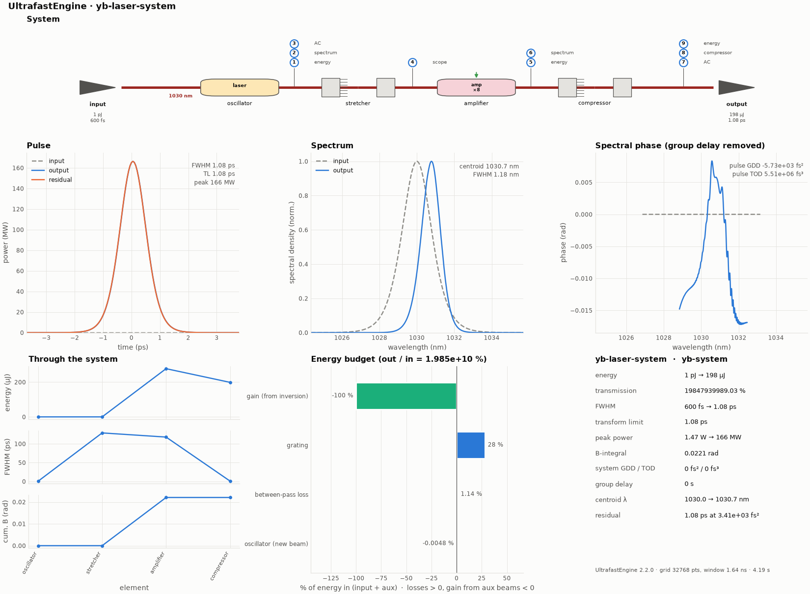
20 -- A complete Yb laser system: oscillator → stretcher → amplifier → compressor¶

ultrafast run system.ufs run.json -o results ultrafast-plot results # system, oscillator, gain, instruments ...

Nonlinear¶

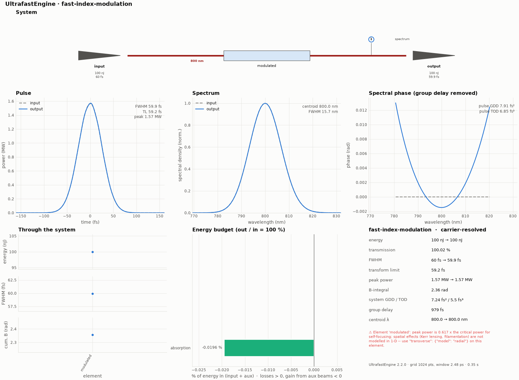
06 -- Carrier-resolved propagation (index varying on the optical-cycle scale)¶

The time response in fast-index.ufs is written in lab time (t_lab) and oscillates at 60 THz.

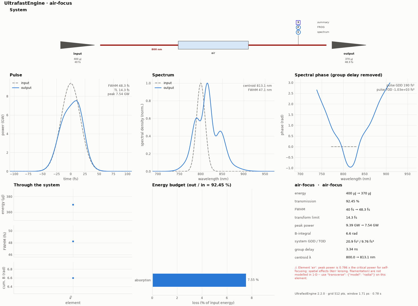
24 -- Air at a focus: rotational Raman, ionisation and pulse retrieval¶

A 0.4 mJ, 40 fs pulse at 800 nm focused (w0 = 100 µm) in the middle of 1 m of air.

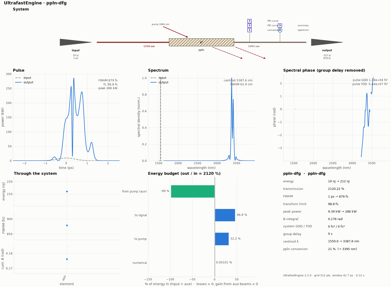
10 -- Mid-IR difference-frequency generation in MgO:PPLN¶

A 1064 nm pump (1 uJ, 1 ps) and a 1550 nm signal (10 nJ) generate a 3.39 um idler in 5 mm of periodically poled MgO:LiNbO3 (type 0, all extraordinary, d33).

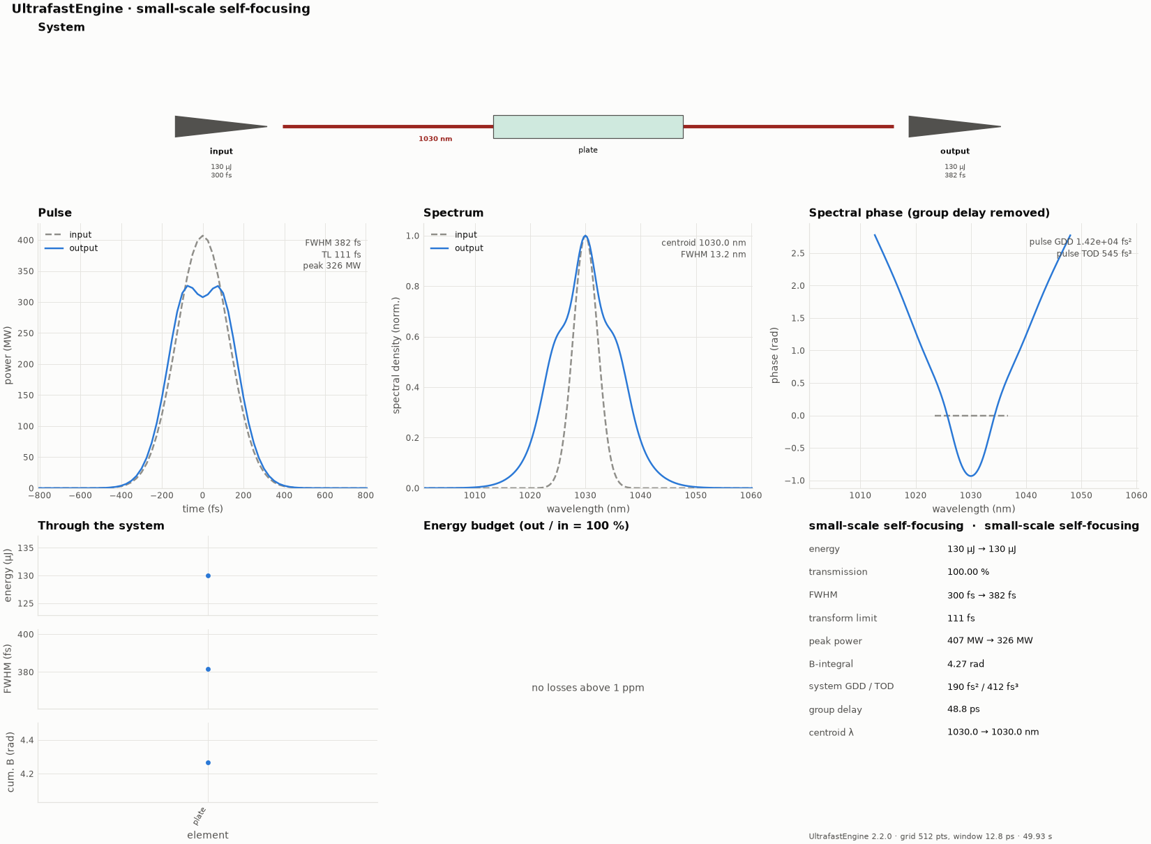
29 -- Small-scale self-focusing in a 2-D plate (P / P_cr ≈ 100)¶

A 300 fs, 130 µJ pulse crosses 10 mm of fused silica in a flat-top beam of radius 0.3 mm: 3.3·10⁸ W, about 100 times the critical power for self-focusing.

Diffraction¶

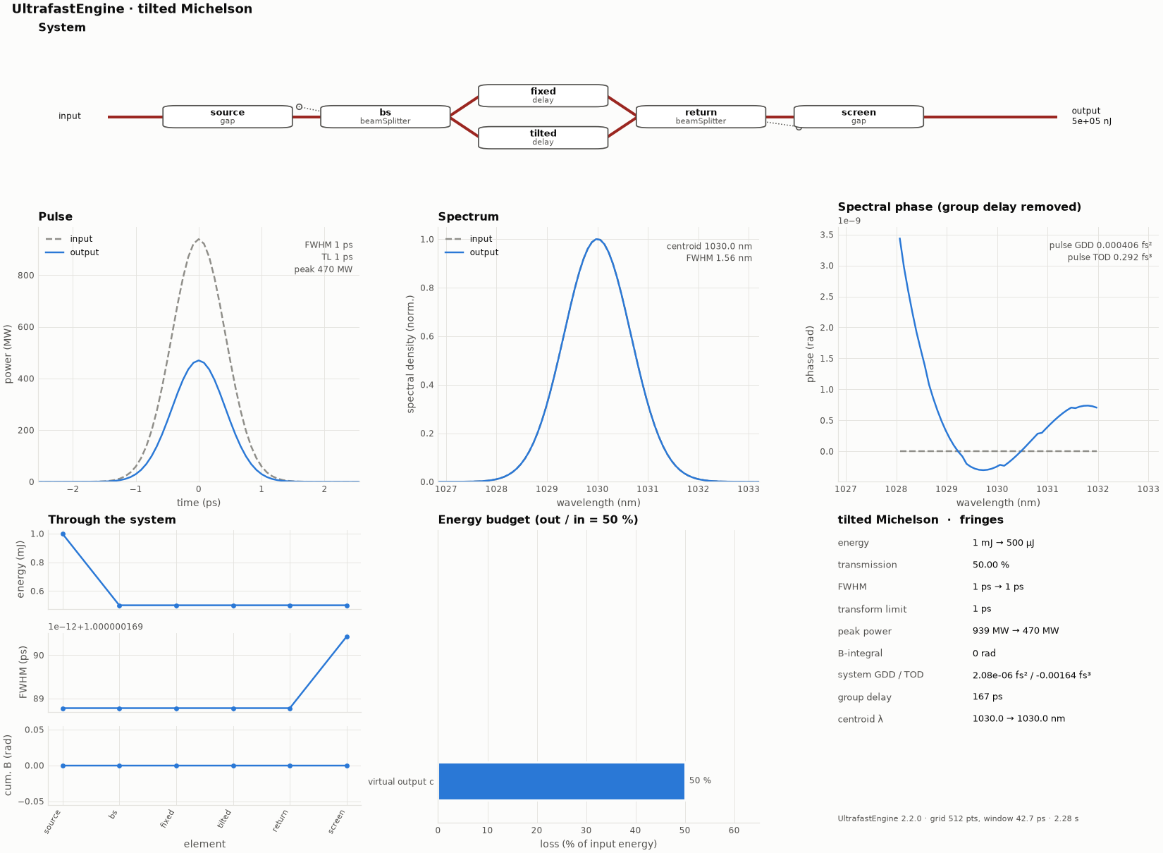
35 -- Fringes from a tilted mirror¶

A Michelson interferometer on the command line, in a Branched .ufs file.

Wavefronts¶

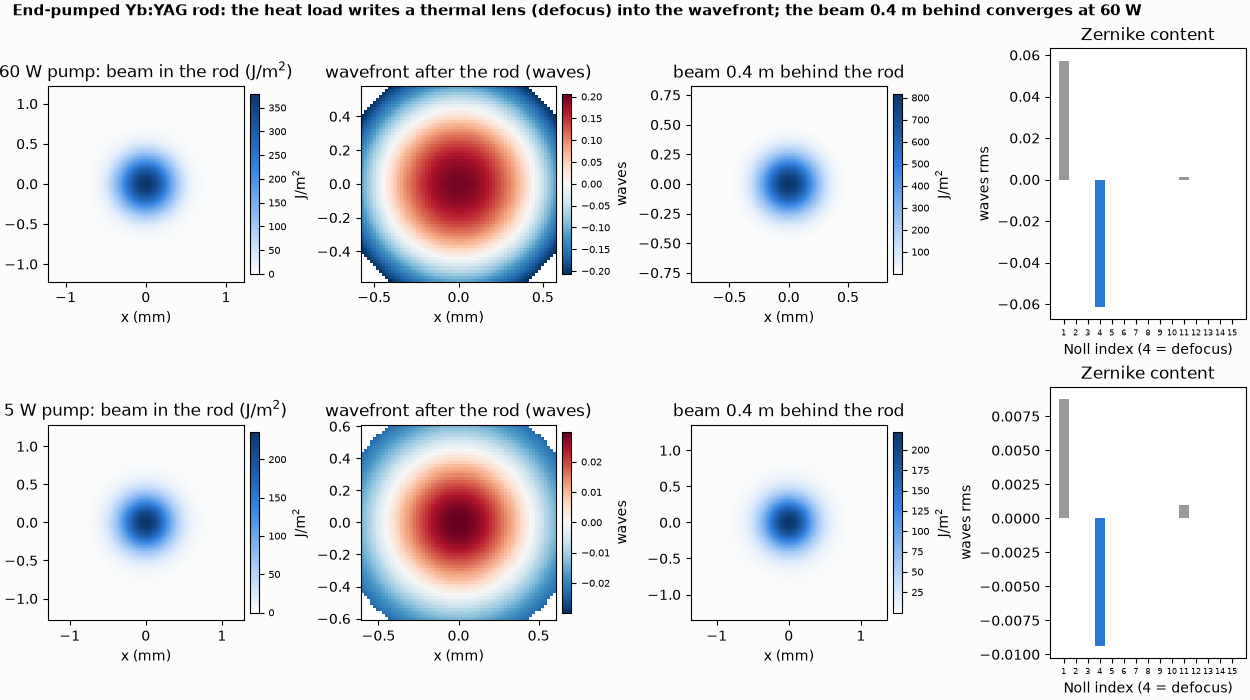
16 -- Position-dependent material properties¶

indexProfile, absorptionProfile and n2Scale make any material property a function of position (x, y, z, r, θ).

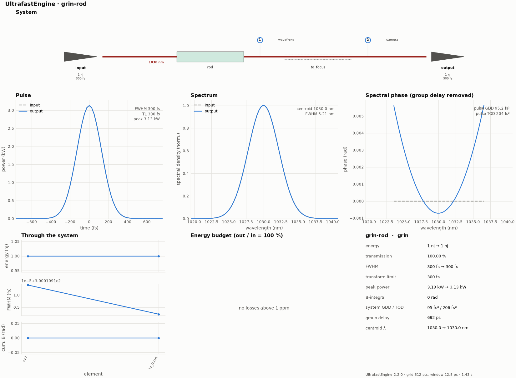
15 -- Spatially resolved gain and the thermal lens¶

A 2 ps, 100 µJ pulse at 10 kHz crosses a 4 mm Yb:YAG rod once, end-pumped by 60 W at 940 nm (super-Gaussian, 0.6 mm, double pass).

Diagnostics¶

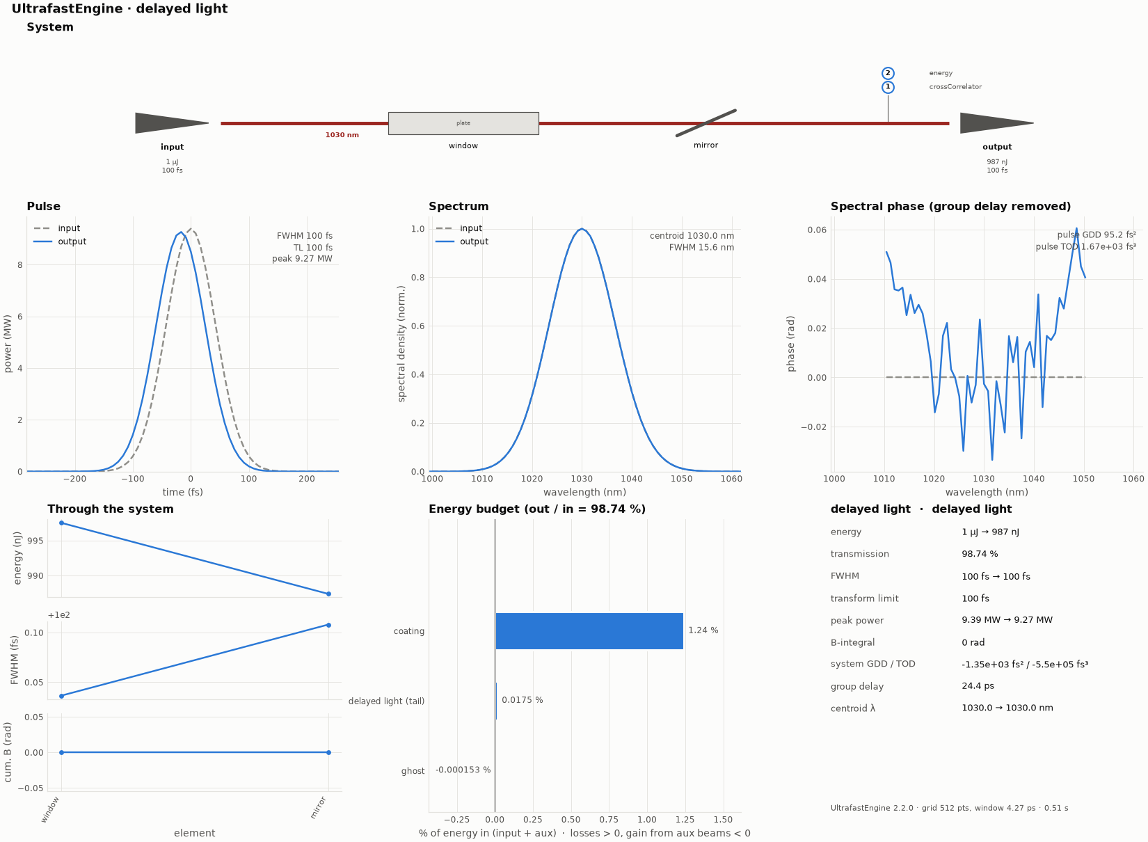
28 -- Delayed light: a plate ghost, a mirror-substrate echo and a coating pedestal on the tail grid¶

A 100 fs pulse passes a fused-silica window with a wavelength-dependent AR coating and reflects from an HR mirror on a 12.7 mm substrate.

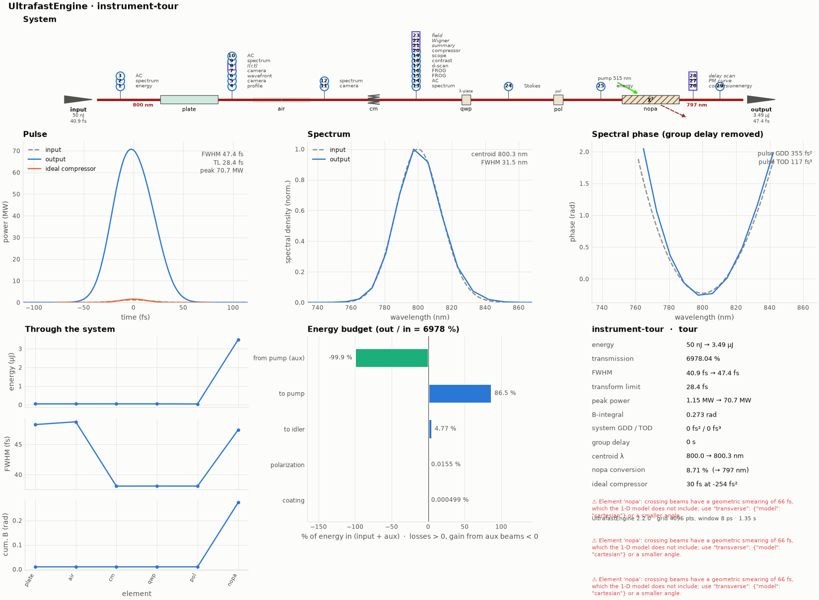
17 -- A tour of every instrument¶

Every instrument kind used once along one beam line.

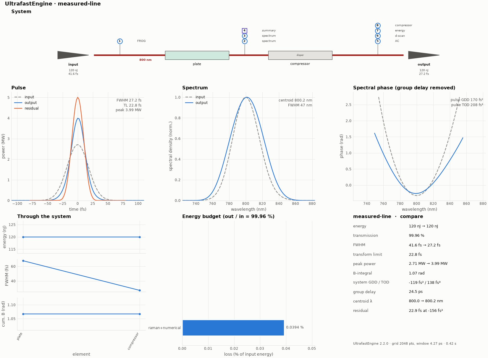
21 -- Measured data: compare, calibrate, predict¶

You have a few-cycle line in the lab and some recorded diagnostics.

Components¶

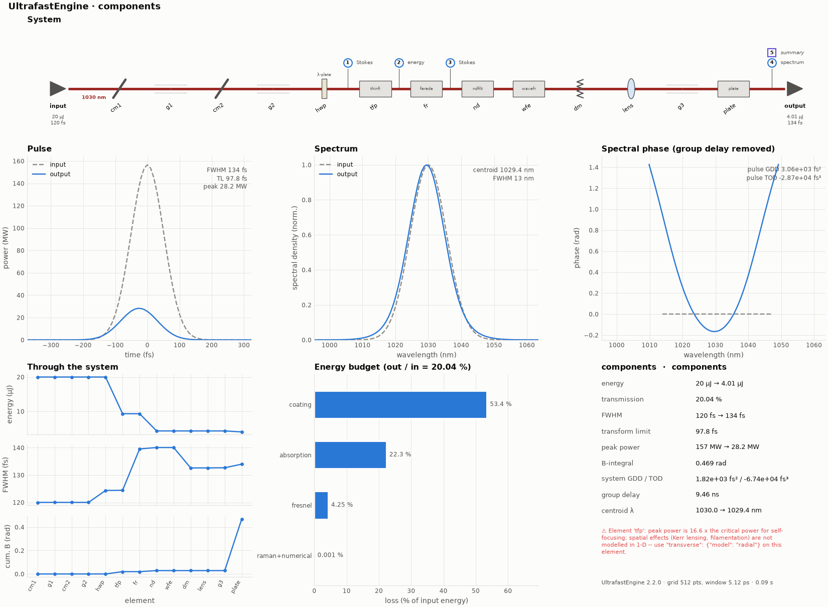
23 -- Optical components and beam tracking¶

One beam line with the optical-component models (Optical components).

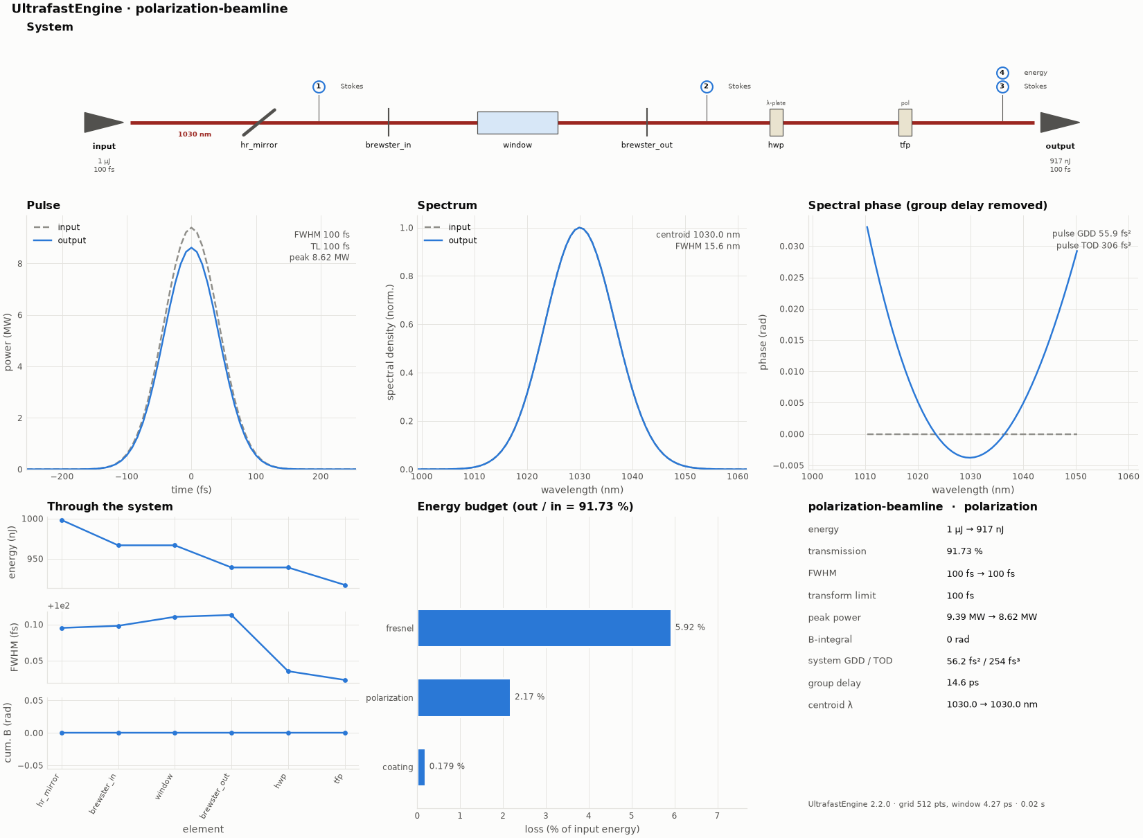
05 -- Polarisation, coatings and Fresnel losses¶

Jones calculus with s/p decomposition at every surface.

Computing¶

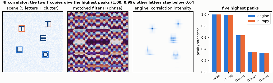
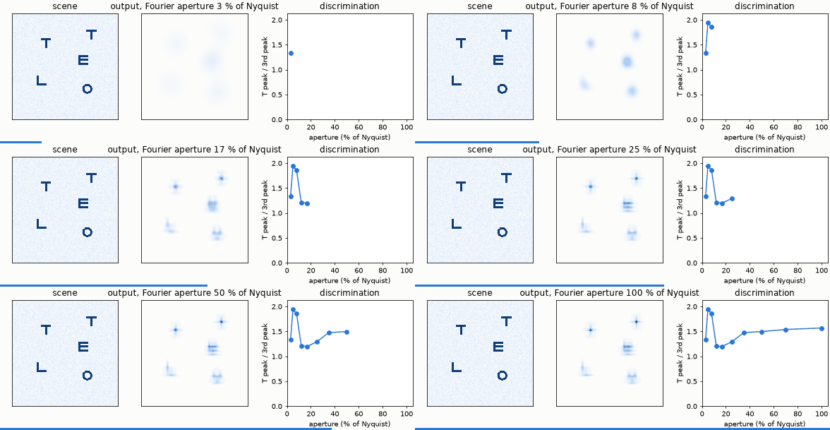
4f correlator¶

A scene of five letters on a clutter background, and a matched filter for the letter T in the Fourier plane of a 4f system.

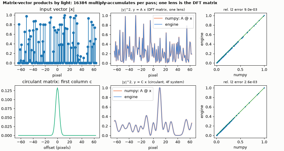
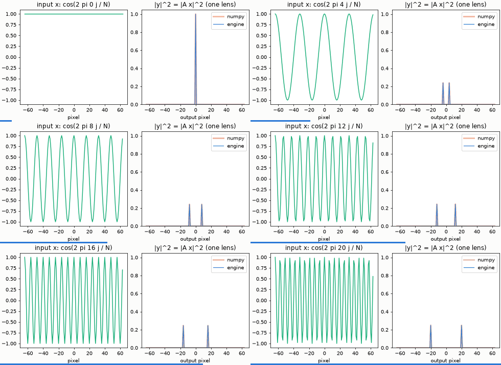
Matrix-vector multiplication by light¶

y = A x with A a fixed matrix and x a vector of N complex numbers written on N pixels (amplitude and phase).

Optical convolution¶

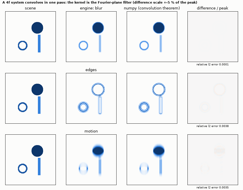
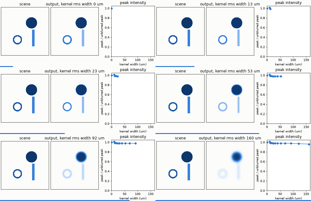
The same 4f layout as a convolution engine.

Parallelism and time¶

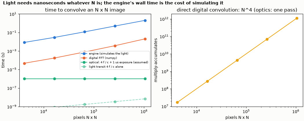
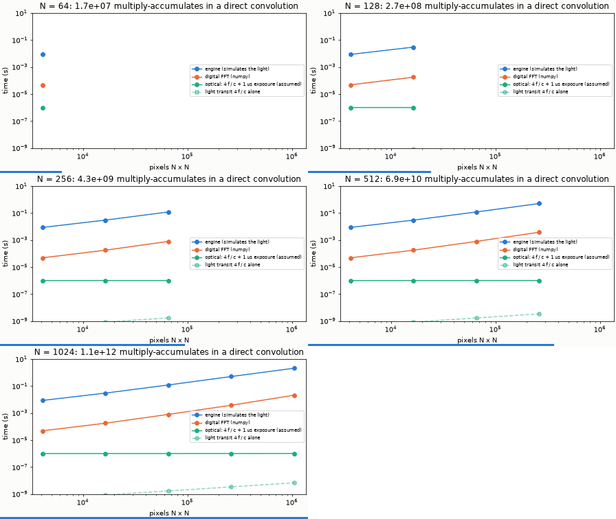
The same Gaussian blur on N x N pixels (pitch 20 µm; the aperture and the focal length f = N dx² / λ grow with N), done three ways: by the engine, by numpy (two FFTs and a product: the digital way), and "optically" (the light crosses 4 f once, plus an assumed sensor exposure).

AdaptiveOptics¶

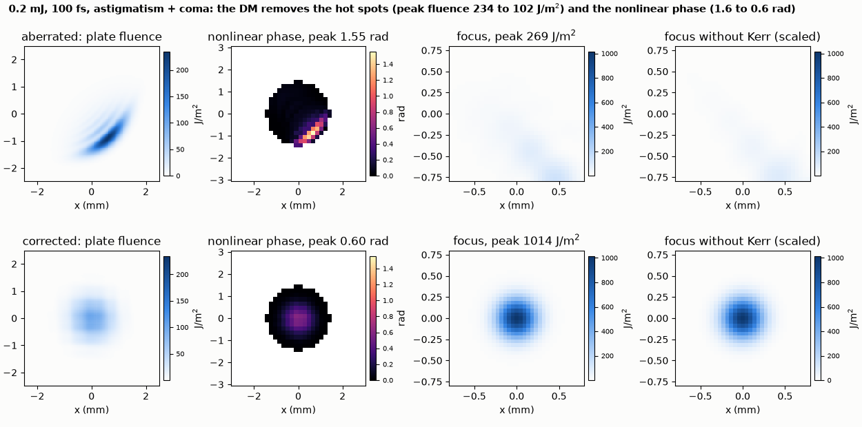
An aberrated high-power beam: what a deformable mirror does for the nonlinear phase¶

A deformable mirror removes the hot spots of an aberrated 2 GW beam and cuts the peak nonlinear phase in a Kerr plate from 1.55 to 0.60 rad.

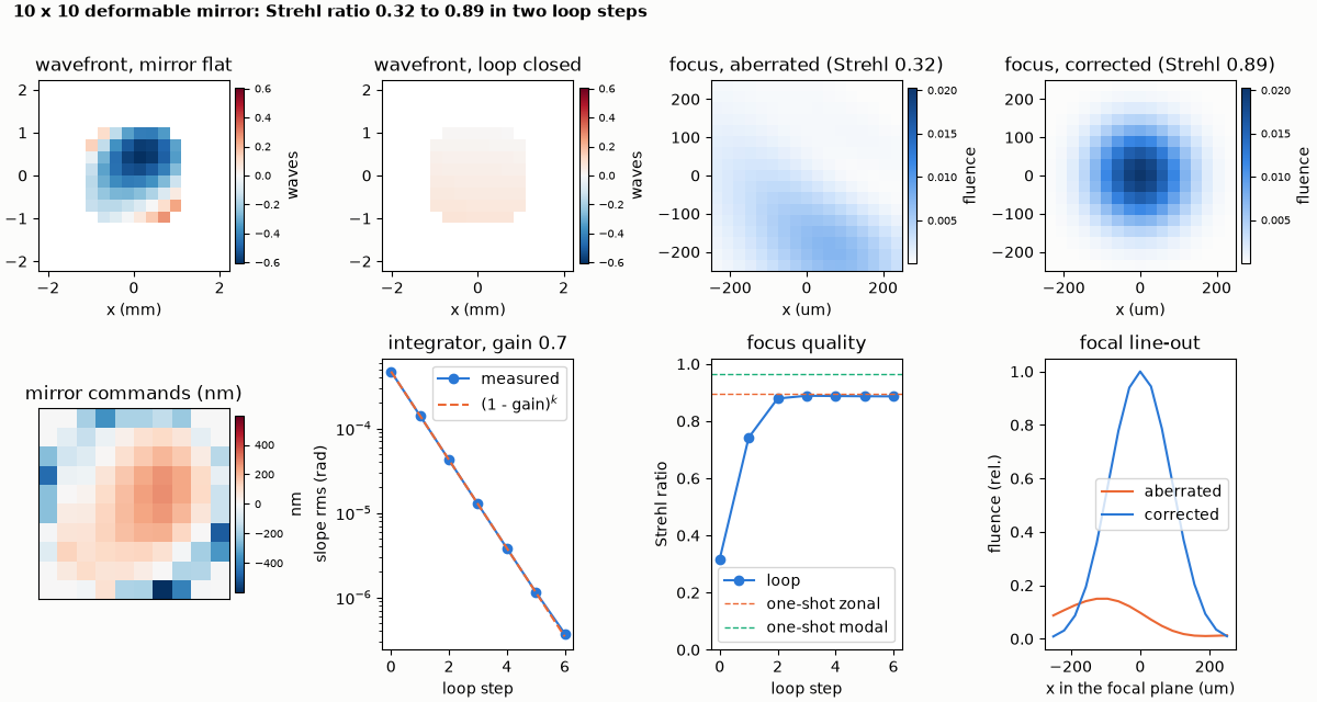
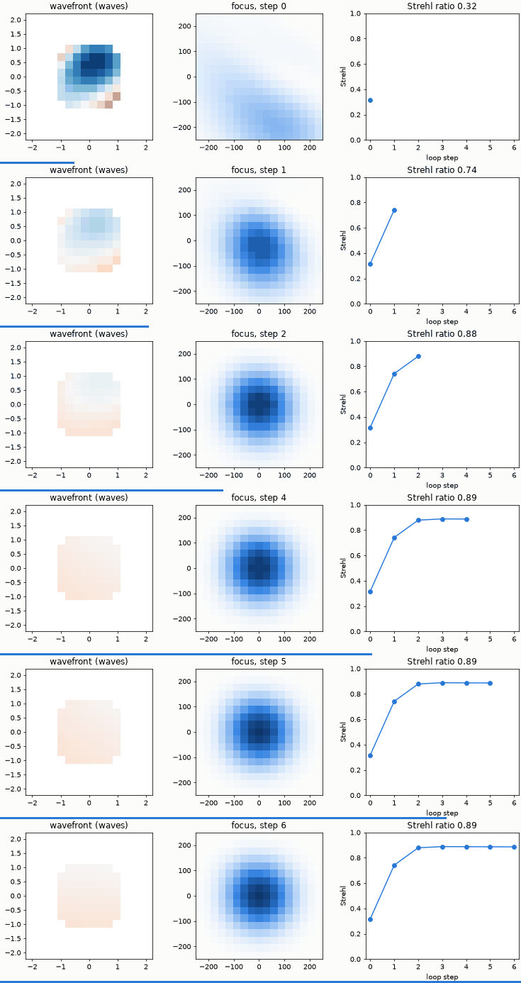
Deformable-mirror correction of an aberrated focus¶

A 10 x 10 deformable mirror, calibrated and run in a closed loop, restores the focus of a beam with defocus, astigmatism and coma (Strehl 0.32 to 0.89).

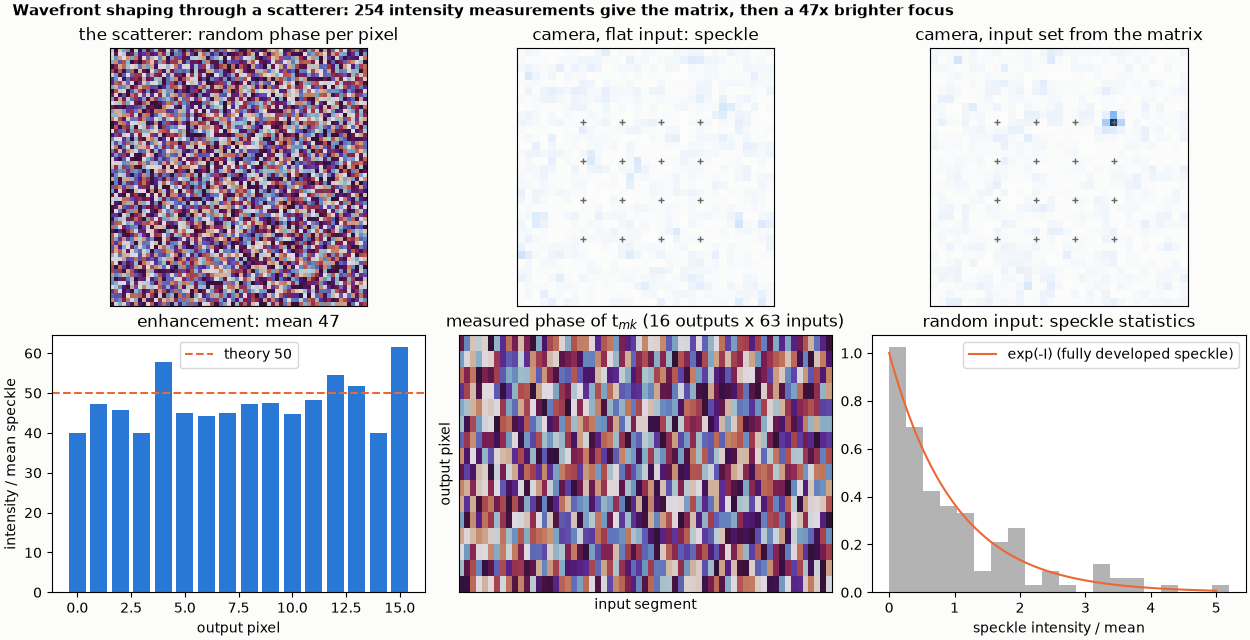
Focusing through a scatterer by wavefront shaping¶

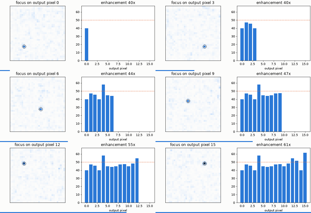
Wavefront shaping measures a scatterer's transmission matrix from intensities alone and turns speckle into a focus about 47 times brighter.

Sensorless adaptive optics¶

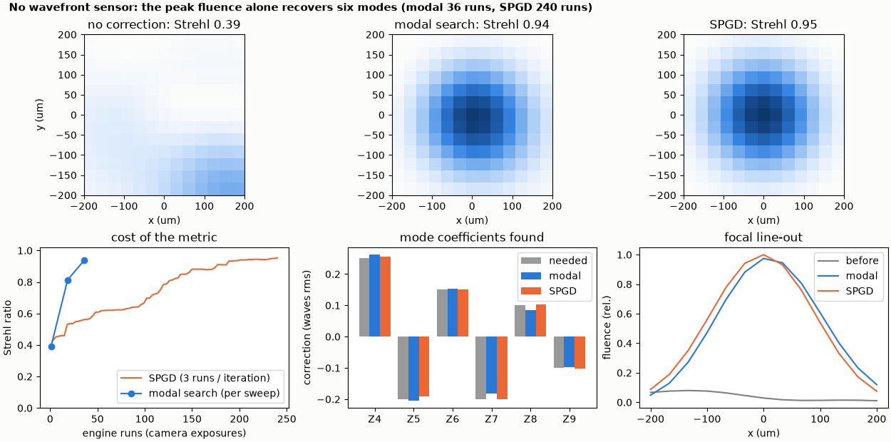
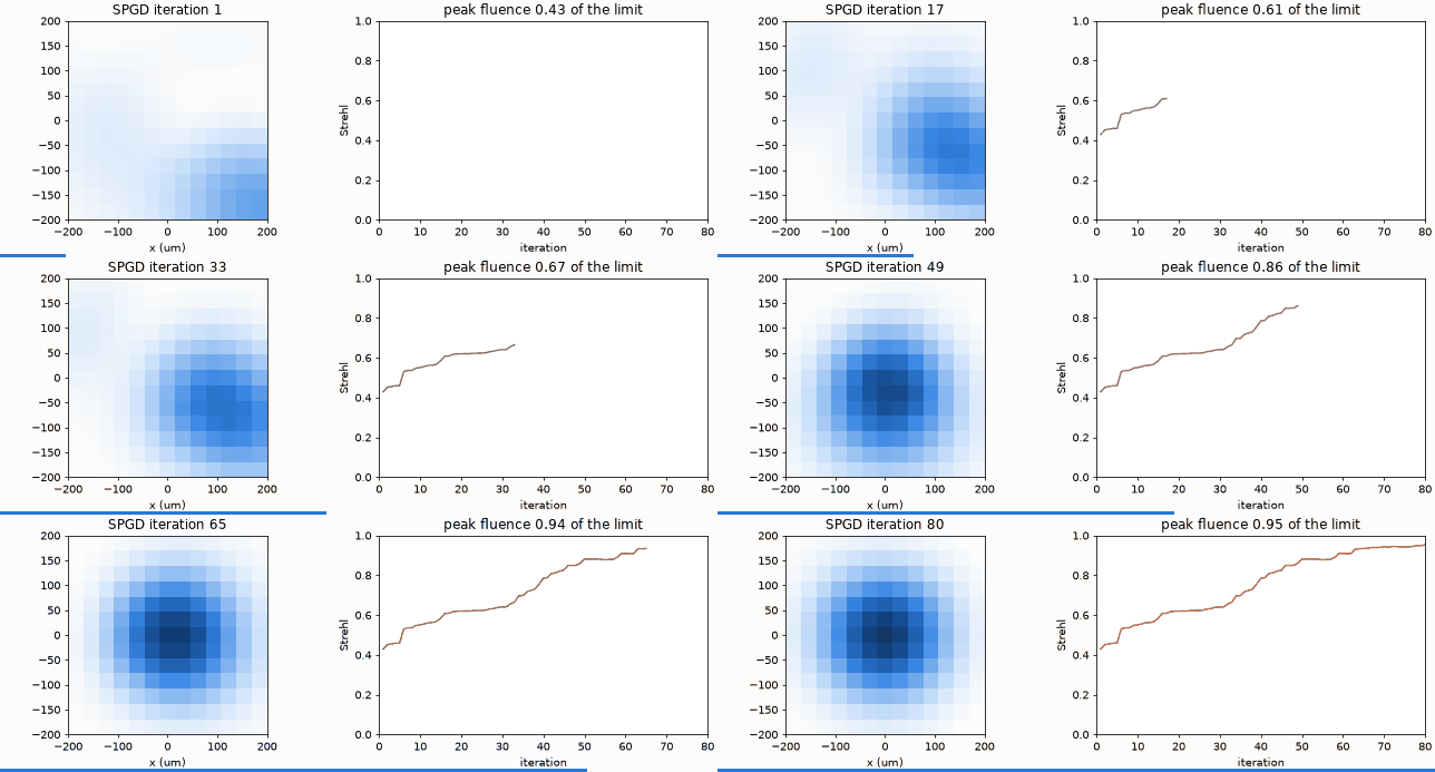
With only the focal peak as a metric, modal search (36 camera exposures) and SPGD (240) improve a six-mode aberration from Strehl 0.39 to 0.94.

Beam shaping with a phase-only SLM¶

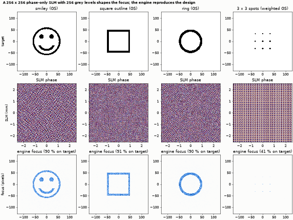
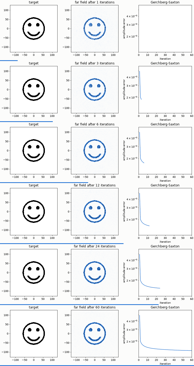
A phase-only SLM with 256 grey levels turns a Gaussian beam into a smiley, a square, a ring and a spot array (Gerchberg-Saxton holograms), up to a full 1920 x 1080 panel.

Temporal pulse shaping¶

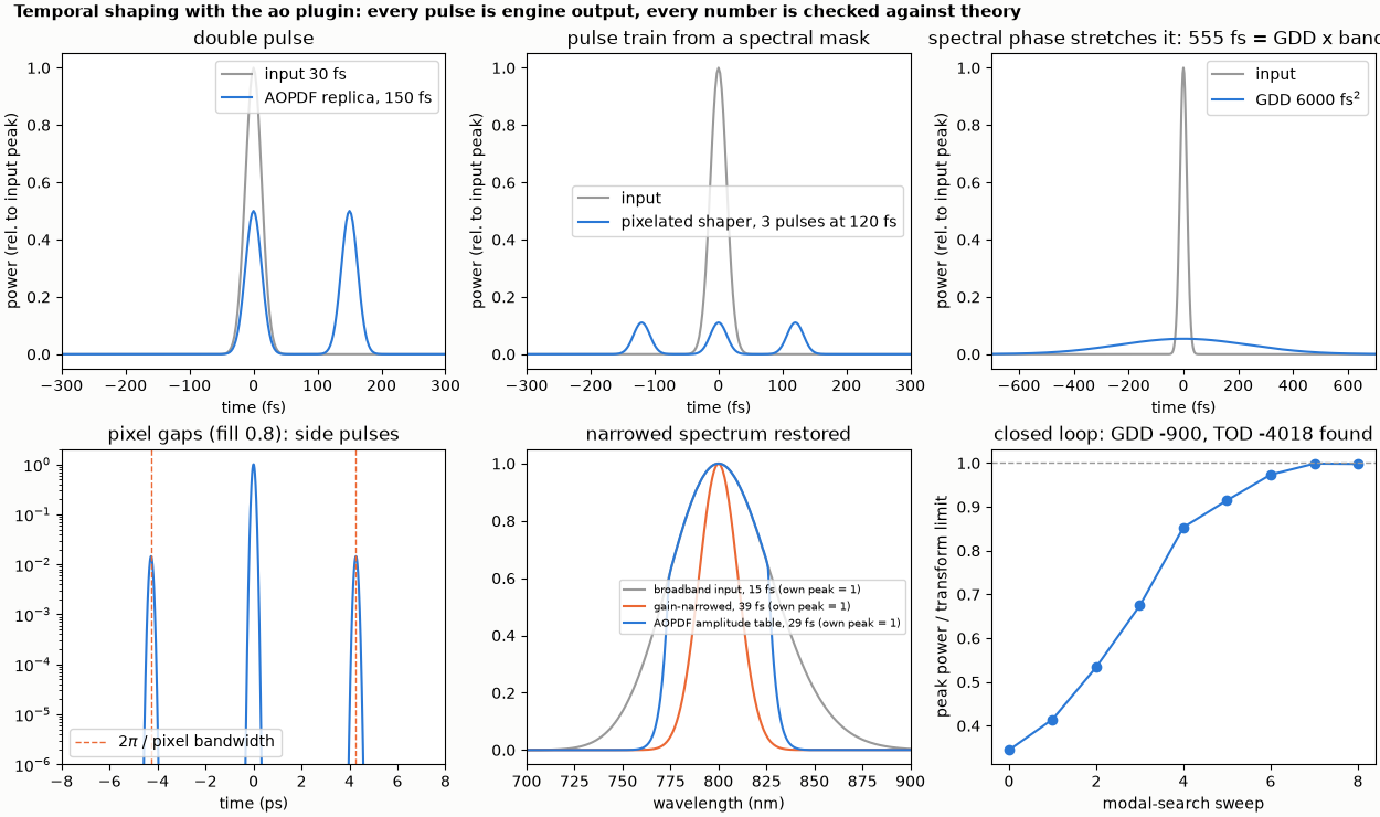
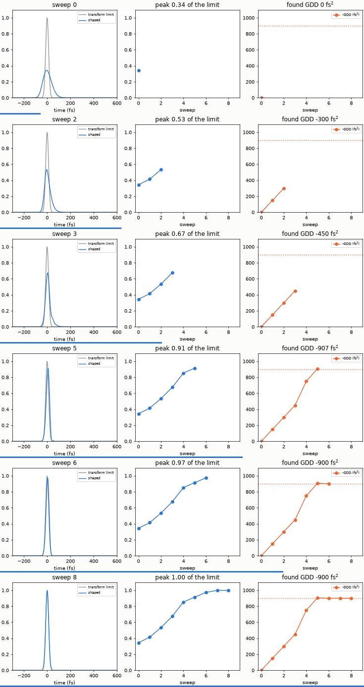
A spectral shaper and an AOPDF make double pulses and pulse trains, show the side pulses of pixel gaps, restore a narrowed spectrum and find an unknown chirp in a closed loop.

Coherent tiled-aperture combining¶

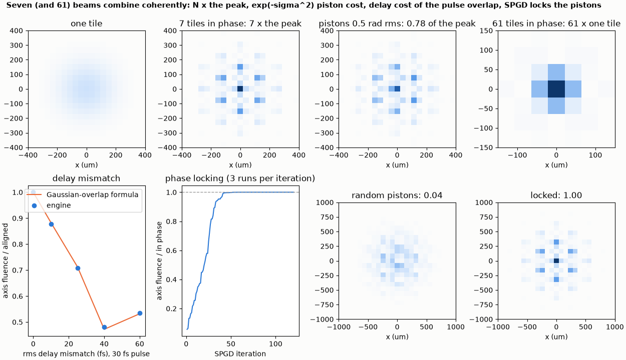
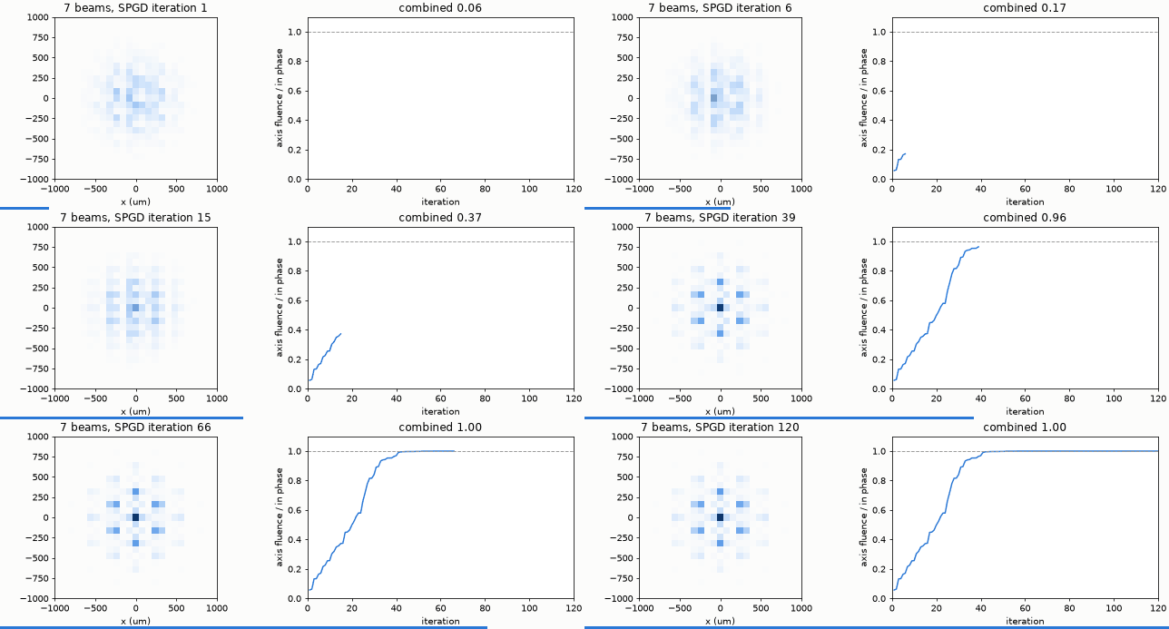
Seven and 61 coherent beams combine to N times the peak; piston and delay errors cost what theory says, and SPGD locks the phases.

DigitalTwin¶

Build a digital twin: fit across conditions, predict, validate¶

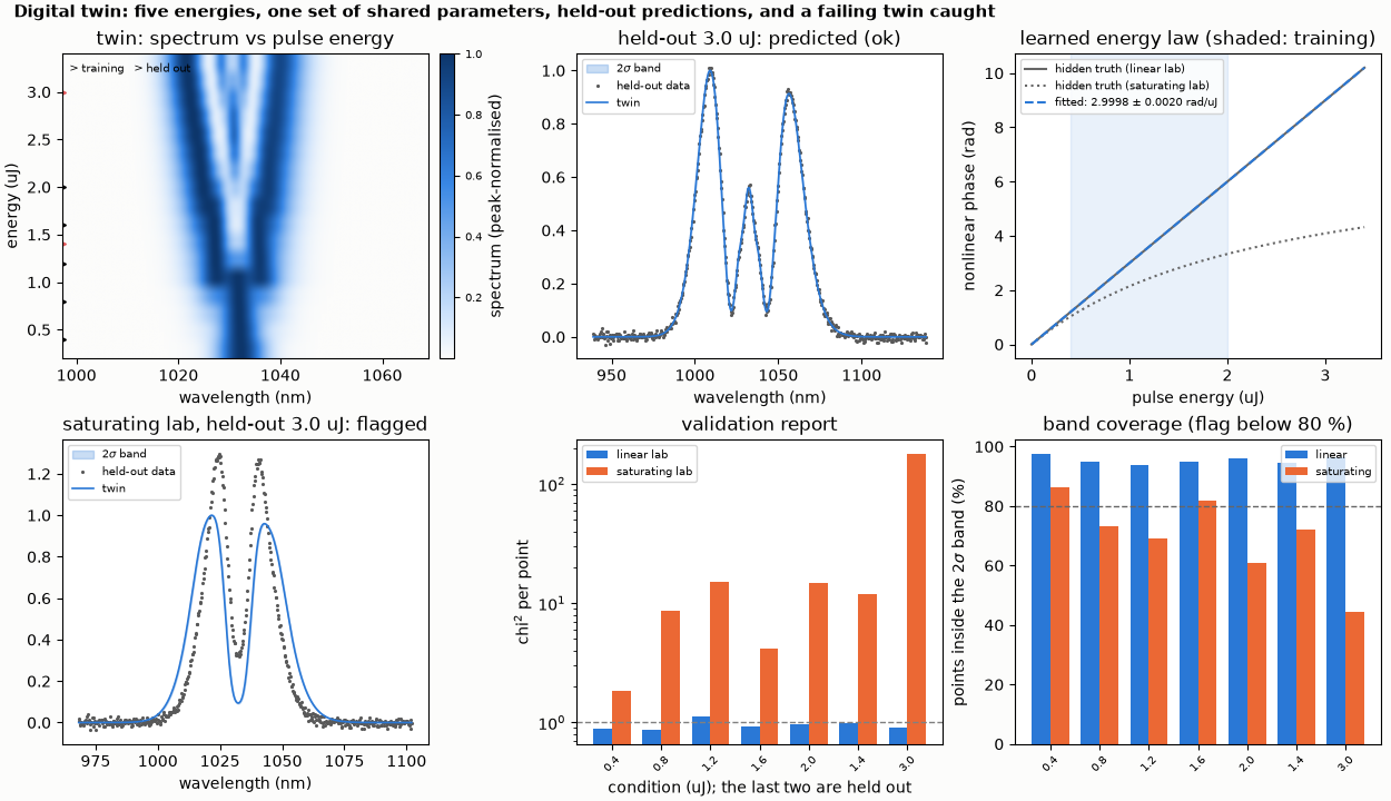
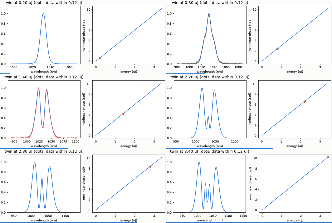
A digital twin fitted to spectra at five pulse energies recovers the hidden filter and nonlinear phase, predicts two held-out energies with credible bands, and flags a twin that only fits its training data.

Explore the twin without beam time¶

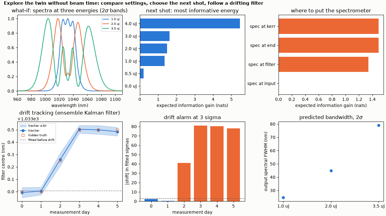
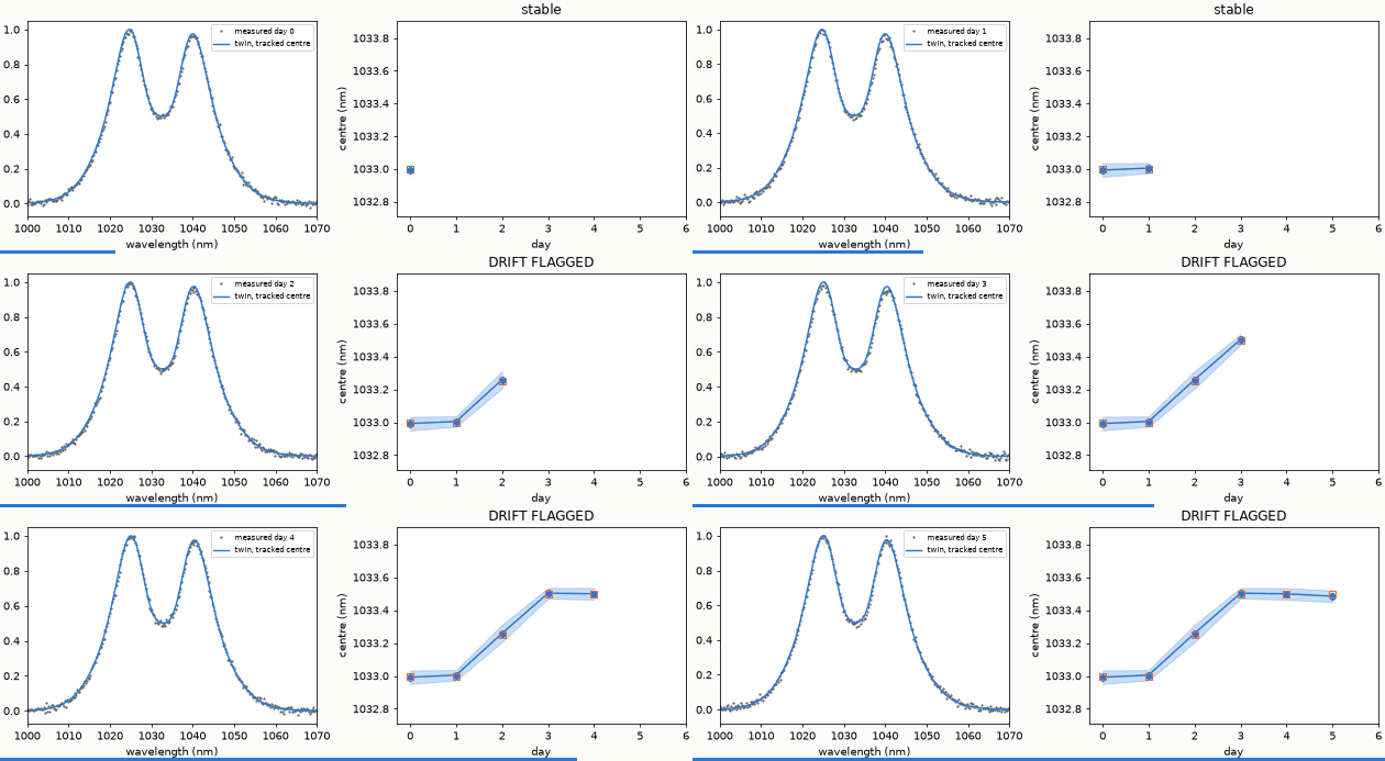
A fitted twin answers what-if questions with credible bands, ranks the next measurement by information gain and follows a drifting filter with an ensemble Kalman filter.

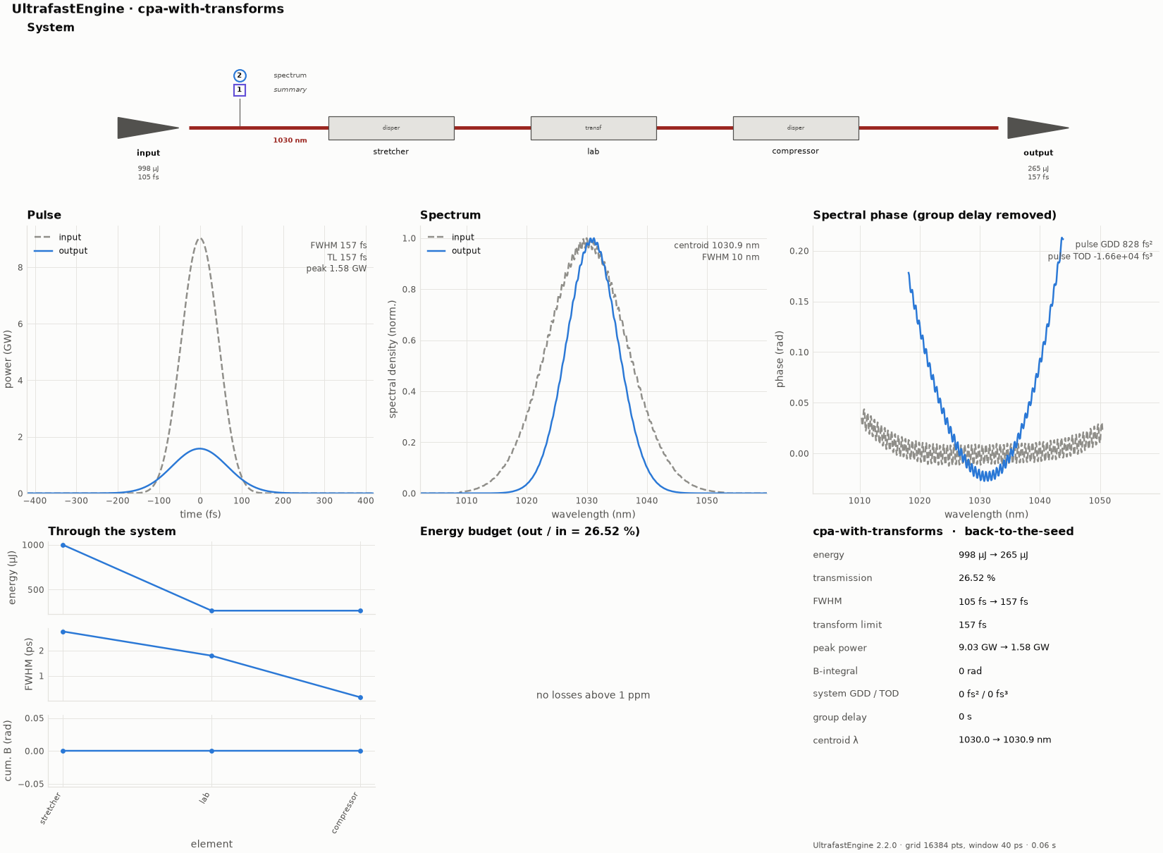
26 -- Transforms: fit what the design does not know, then reuse it¶

A CPA line on paper: a stretcher (+100 000 fs², −300 000 fs³) and a compressor that undoes it exactly.

Fibres¶

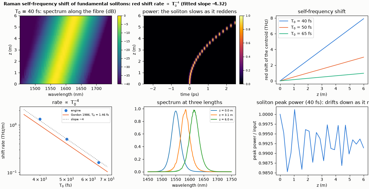
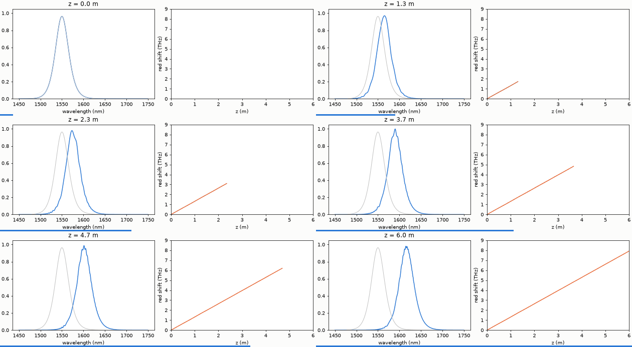
Raman self-frequency shift of solitons¶

Raman scattering pushes fundamental solitons to the red at a rate proportional to T0^-4 (Gordon 1986); the engine reproduces the scaling.

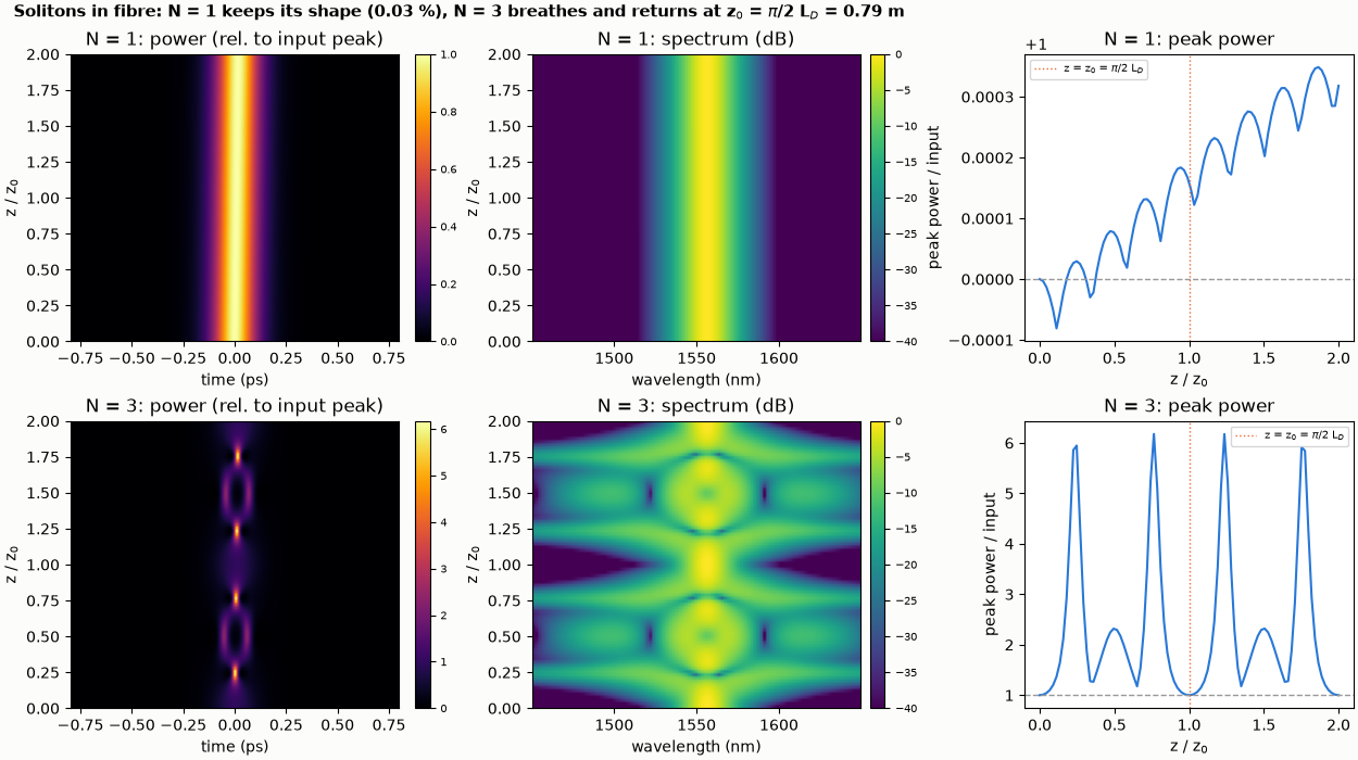
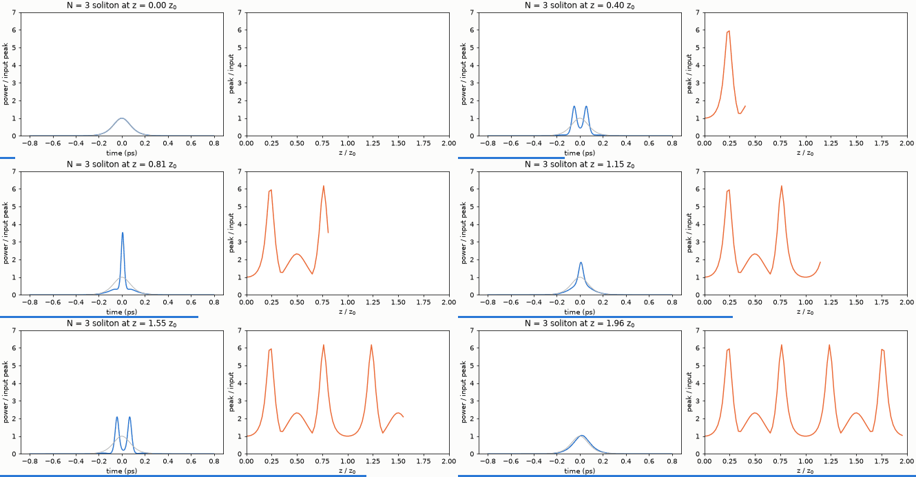
Solitons in a fibre: shape-keeping and breathing¶

An N = 1 soliton keeps its shape and an N = 3 soliton breathes and returns after exactly one soliton period z0 = (pi/2) L_D.

Nonlinear pulse compression in a fibre¶

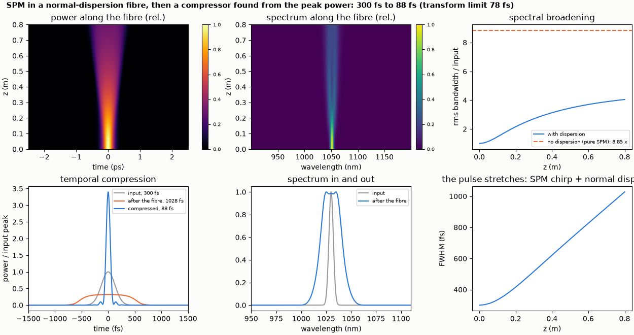
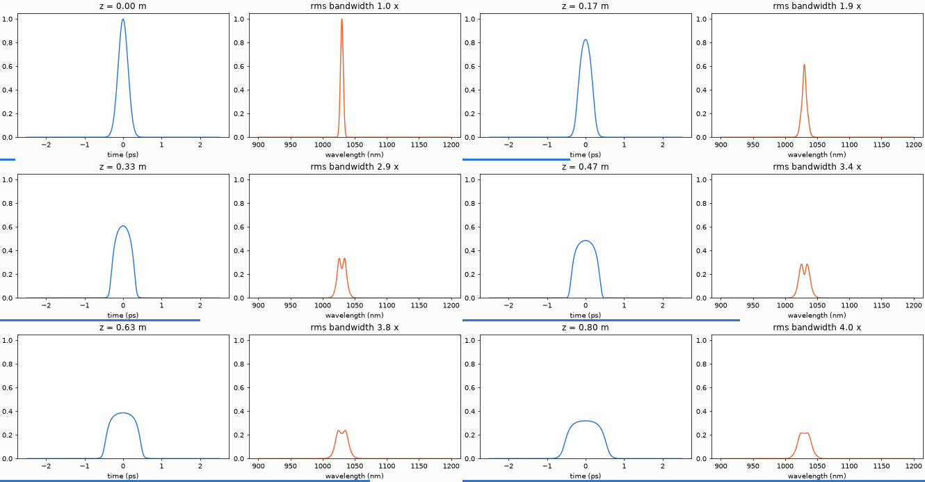
Self-phase modulation in a normal-dispersion fibre and a compressor found from the peak power alone shorten a 300 fs pulse to 88 fs.