
21 -- Measured data: compare, calibrate, predict
You have a few-cycle line in the lab and some recorded diagnostics. This example shows how to:
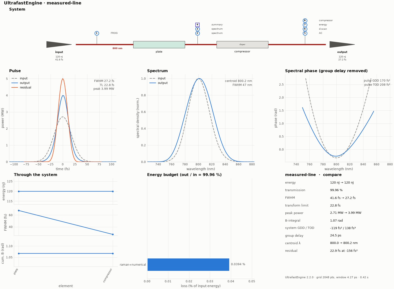
The overview figure of this example's run (python make_figures.py redraws it; the file is hero.png).
- compare the model with your recordings (
run-compare.json); - calibrate the numbers you do not know well by fitting them to all the recordings at once (
run-fit.json); - predict, with error bars, what instruments you do not have would show.
The line (line.ufs): a chirped 25 fs, 800 nm pulse is focused to 40 µm into a 5 mm fused-silica plate (SPM and a
weak Kerr lens, radial grid), then recompressed by a compressor modelled as pure GDD. Three numbers are uncertain:
the input chirp, the pulse energy and the compressor GDD. Our first guesses are 300 fs², 120 nJ and −300 fs².
cd docs/examples/Diagnostics/measured-data
ultrafast run line.ufs run-compare.json -o results-compare     # model vs data, a few seconds
ultrafast run line.ufs run-fit.json     -o results-fit         # calibration, ~2 minutes (45 runs)
ultrafast-plot results-fit                                     # plots/measurements.png and plots/fit.png
The recorded data (data/)
| file | instrument | format |
|---|---|---|
fibre_spectrum.csv |
fibre-coupled spectrometer: a 50 µm core in the focal plane of an f = 100 mm lens after the plate | CSV, columns wavelength_nm,counts; raw counts with a ~30-count dark background and shot noise |
autocorrelation.csv |
intensity autocorrelator after the compressor | CSV, delay_fs,signal; 1 % noise |
dscan.npz |
d-scan with fused-silica wedges after the compressor | NPZ with insertion_mm (31), wavelength_nm (121) and trace (31 × 121); 2 % noise |
power_meter.json |
power meter after the compressor | {"energyJ": 1.441e-07}; 3 % calibration uncertainty |
The units come from the column names (_nm, _fs, _mm, ... see Measured data).
In real life these files come from your lab. Here make_data.py generated them from the same model with the
true values (450 fs², 140 nJ, −520 fs²), then added noise and a background. Rerun it to regenerate them.
1. Compare: run-compare.json
Each instrument with recorded data gets a "measured" block:
{ "kind": "spectrometer", "name": "fibre_spectrum", "at": "plate", "resolutionM": 1e-9,
  // what the fibre sees: the far field of the plate output, through a 25 um radius core
  "sampling": { "plane": "far", "focalLengthM": 0.1, "aperture": { "kind": "fibre", "radiusM": 25e-6, "na": 0.22 } },
  "measured": { "file": "data/fibre_spectrum.csv", "background": "auto", "sigma": 0.03 } },
{ "kind": "autocorrelator", "name": "ac_out", "at": "end",
  "measured": { "file": "data/autocorrelation.csv", "sigma": 0.02 } },   // or just "measured": "data/autocorrelation.csv"
{ "kind": "dscan", "name": "dscan_out", "at": "end", "material": "FusedSilica", "insertionM": [-3e-3, 3e-3], "steps": 31,
  "measured": { "file": "data/dscan.npz", "sigma": 0.03 } },
{ "kind": "powerMeter", "name": "power_out", "at": "end",
  "measured": { "file": "data/power_meter.json", "valueSigma": 0.03 } }
The simulated reading is interpolated onto the measured axis and both are normalised (by default the simulation to its peak, with the data scaled onto it by least squares). The run reports a χ² and an rms error per instrument:
  measured data:
    fibre_spectrum         spectrometer   chi^2 37.38      (401 points)  rms error 0.92 %
    ac_out                 autocorrelator chi^2 262.8      (201 points)  rms error 2.29 %
    dscan_out              dscan          chi^2 9017       (3751 points)  rms error 4.65 %
    power_out              energyMeter    chi^2 31.27      (1 points)
      energyJ: measured 1.441E-07 +- 4.3E-09, simulated 1.2E-07 (-5.6 sigma)
The first guesses are clearly off: the d-scan and the power meter disagree with the model. measurements.png shows
every comparison: the curves with their residuals, the measured and simulated d-scan and their difference, and the
scalar readings in units of σ.
2. Calibrate: run-fit.json
The same instruments, plus a "fit" block that names the uncertain numbers by their path in the run or system
file:
"fit": {
  "parameters": [
    { "name": "input chirp",    "path": "pulse/chirp/gddFs2",          "min": -500,  "max": 1500,  "unit": "fs^2" },
    { "name": "input energy",   "path": "pulse/energyJ",               "min": 50e-9, "max": 300e-9, "unit": "J" },
    { "name": "compressor GDD", "path": "element:compressor/gddFs2",   "min": -1500, "max": 0,     "unit": "fs^2" }
  ],
  "maxIterations": 20
}
The fit (Levenberg–Marquardt) minimises the total χ² over every measured instrument:
fit: calibrate parameters against the measured instruments ...
  fit: chi^2 9346 -> 1611 (4354 points, reduced 0.37), 5 iterations, 25 runs
  input chirp                               463.968 +- 9.01         (start 300)
  input energy                          1.42969E-07 +- 3.74E-09     (start 1.2E-07)
  compressor GDD                           -533.69 +- 8.13         (start -300)
  fibre_spectrum                     rms error 0.92 % -> 0.76 %
  ac_out                             rms error 2.28 % -> 0.92 %
  dscan_out                          rms error 4.65 % -> 1.92 %
  power_out                          chi^2 31.3 -> 0.0758
  WARNING: Fit: parameters input chirp and compressor GDD are strongly correlated (-0.989): ...
| parameter | first guess | fitted (±1σ) | true | deviation |
|---|---|---|---|---|
| input chirp | 300 fs² | 463 ± 9 fs² | 450 fs² | 1.4σ |
| input energy | 120 nJ | 142.5 ± 3.7 nJ | 140 nJ | 0.7σ |
| compressor GDD | −300 fs² | −533 ± 8 fs² | −520 fs² | 1.6σ |
| net GDD (chirp + compressor) | 0 | −69.8 fs² | −70 fs² |
All three are recovered within 2σ (the net GDD, the best-determined combination, to 0.2 fs²), and the residuals left after the fit are at the noise level of the data. The reduced χ² of 0.37 means the stated σ (3 %) is larger than the actual noise (about 2 %), so the error bars are conservative.
Why the correlation warning? The autocorrelator and the d-scan sit after the compressor, so they mostly measure
the net GDD. That is fixed to about ±1.5 fs². Only the spectrum after the plate distinguishes the input chirp from
the compressor, through how much SPM the chirped pulse makes in the plate, and that is a weaker handle. The fit
therefore says: the sum is well known, the split less so (±9 fs²). To pin down the split, add an instrument before
the compressor, such as an autocorrelator or FROG at plate.
The energy is correlated with the chirp (+0.85) for a similar reason: more energy and more chirp can produce the same SPM. The power meter breaks that tie.
fit.png shows the fitted values, the cost per iteration, the correlation matrix and χ² per instrument before and
after. fit.json holds everything, including the covariance.
3. Predict
After the fit, every instrument and element value is reported with a 1σ uncertainty, propagated from the parameter
covariance (fit.json → predictions). This includes instruments that have no data:
| prediction | value ± σ | true |
|---|---|---|
pulse after the plate, FWHM (after_plate.fwhmS) |
83.7 ± 1.1 fs | 82.9 fs |
spectrum after the plate, FWHM (after_plate.spectralFwhmM) |
46.99 ± 0.19 nm | 46.97 nm |
B-integral in the plate (plate.bIntegralRad) |
0.966 ± 0.020 rad | 0.966 rad |
input FROG delay marginal, FWHM (frog_input.delayMarginalFwhmS) |
79.9 ± 1.3 fs | 79.0 fs |
GDD still to remove at the end (residual.compressorGddS2) |
−85.7 ± 1.5 fs² | −85.7 fs² |
best compressed FWHM (residual.compressedFwhmS) |
23.77 ± 0.02 fs | 23.84 fs |
output FWHM (compressor.fwhmS) |
25.13 ± 0.06 fs | 25.13 fs |
fibre coupling (fibre_spectrum.samplingTransmission) |
0.296 % |
The error bars are 1σ from the linearised parameter covariance. The compressed FWHM is so tightly constrained (±0.02 fs) that the 0.07 fs difference from the true value is ~3σ. That is the limit of a linear error estimate on a quantity that depends weakly, and nonlinearly, on the parameters.
The plots show these as ±1σ bands on the simulated curves (<instrument>_simulated_sigma in result.npz).
Things to try
- Delete
power_out: the energy is then fixed only by the SPM, through its correlation with the chirp. Watch how its σ changes. - Extend
make_data.pyto write an autocorrelation atplateas well, add it with"measured", and watch the chirp/compressor correlation drop. - Use the integrated spectrum instead of the fibre spectrum: the fibre in the far field sees a narrower spectrum (43.8 nm vs 47.1 nm), because SPM is strongest on axis and the far field weights the beam differently. Fitting the wrong instrument model biases the chirp.
- Set
"freezeGrid": falsein"fit"to let each run size its own grid (slower, and less smooth for the fit).
See Measured data for every comparison option, the fitting plugin for the fit, and the tutorial for a step-by-step walkthrough with your own data.