26 -- Transforms: fit what the design does not know, then reuse it¶

A CPA line on paper: a stretcher (+100 000 fs², −300 000 fs³) and a compressor that undoes it exactly. In the lab the compressed pulse is 157 fs instead of 100 fs, the spectrum is narrower, and the contrast trace shows a post-pulse and a pedestal. This example:

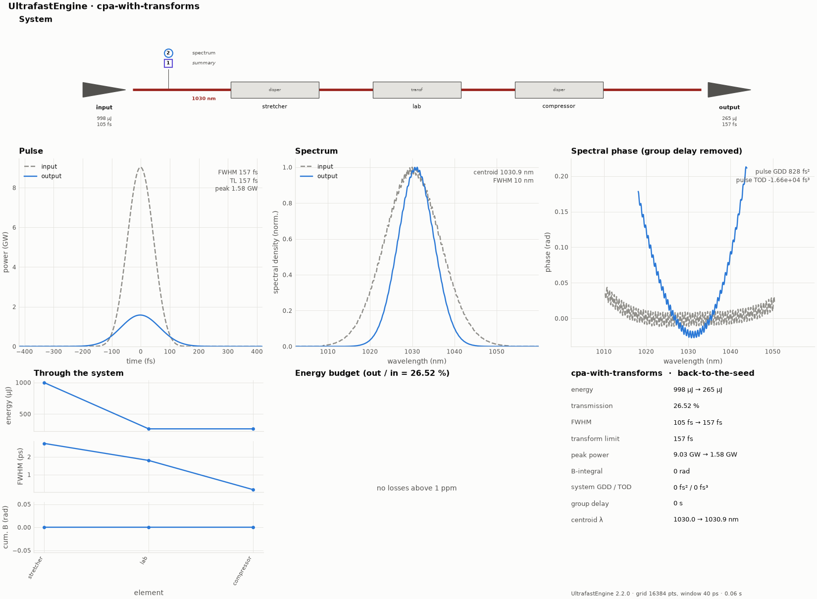
The overview figure of this example's run (python make_figures.py redraws it; the file is hero.png).

1. fits a transform element between stretcher and compressor to four recordings: a spectrum, a d-scan, a third-order cross-correlation and a power reading (run-fit.json);
2. reuses the fitted line on a different seed pulse (run-new-input.json);
3. propagates backward the measured output field to find the seed (run-backward.json).

cd docs/examples/DigitalTwin/transforms
ultrafast run line.ufs run-fit.json -o results-fit                              # ~10 s, 54 runs
ultrafast run results-fit/fitted-system.ufs run-new-input.json -o results-new    # the fitted line, new seed
ultrafast run line.ufs run-new-input.json -o results-design                     # the same seed, unfitted values
ultrafast run results-fit/fitted-system.ufs run-backward.json -o results-backward
ultrafast-plot results-fit                                                      # measurements.png, fit.png

The transform (line.ufs)¶

{ "id": "lab", "type": "transform", "operators": [
    { "kind": "spectralPhase",                                  // residual dispersion of the stretcher/compressor pair
      "gddFs2": { "value": 0, "fit": true, "min": -3000, "max": 3000 },
      "todFs3": { "value": 0, "fit": true, "min": -60000, "max": 60000 },
      "fodFs4": { "value": 0, "fit": true, "min": -2e6, "max": 2e6, "prior": 1e6 } },   // weakly measured: a prior
    { "kind": "spectralAmplitude", "shape": "gaussian",           // gain narrowing
      "fwhmNm": { "value": 20, "fit": true, "min": 5, "max": 60 },
      "centerWavelengthNm": { "value": 1030, "fit": true, "min": 1020, "max": 1040 } },
    { "kind": "energy", "transmission": { "value": 0.5, "fit": true, "min": 0.05, "max": 1 } },
    { "kind": "replica", "delayPs": 6.0,                          // an etalon: the delay is known, the level is not
      "relativeIntensityDb": { "value": -50, "fit": true, "min": -90, "max": -20 } },
    { "kind": "pedestal", "type": "ase", "durationS": 20e-12, "seed": 7,
      "relativeIntensityDb": { "value": -100, "fit": true, "min": -130, "max": -60 } }
] }

Eight numbers are marked with "fit": true. The run spec's "fit" block lists no parameters at all: marked transform numbers are found automatically. The levels are in dB because contrast features span decades.

The recordings (data/)¶

file	instrument	notes
spectrum.csv	spectrometer, 0.2 nm resolution (wavelength_nm,counts)	shot noise and a dark level; "background": "auto", and "resolutionM": 0.2e-9 is checked against the simulated instrument
dscan.npz	d-scan over ±20 000 fs² (gdd_fs2, shg_wavelength_nm, trace)	2 % noise; fixes the sign and size of the residual phase
cross_correlation.csv	third-order cross-correlator (delay_ps,signal_db), 110 dB range	1 dB noise; compared in dB ("scale": "log", "sigmaDb": 1.5) so the −88 dB pedestal counts
power.json	power meter	2 % uncertainty
output_field.csv	the output field (spectrum and phase, as a d-scan retrieval gives it)	for the backward run

make_data.py made them from the same line with the true values, then added noise. Rerun it to regenerate them.

1. Fit¶

  fit (levenbergMarquardt):
  fit: chi^2 9.437E+04 -> 4164 (5344 points, reduced 0.78), 5 iterations, 54 runs
  lab.spectralPhase.gddFs2                  817.811 +- 34.5         (start 0)
  lab.spectralPhase.todFs3                 -16526.4 +- 6.57E+03     (start 0)
  lab.spectralPhase.fodFs4                 -1847.88 +- 8.9E+05      (start 0)
  lab.spectralAmplitude.fwhmNm              13.0161 +- 0.0229       (start 20)
  lab.spectralAmplitude.centerWavelengthNm  1031.51 +- 0.00745      (start 1030)
  lab.energy.transmission                  0.420278 +- 0.00842      (start 0.5)
  lab.replica.relativeIntensityDb          -45.8705 +- 0.291        (start -50)
  lab.pedestal.relativeIntensityDb         -87.9834 +- 0.0851       (start -100)

	true	fitted
GDD	800 fs²	818 ± 34 fs²
TOD	−15 000 fs³	−16 500 ± 6 600 fs³
FOD	400 000 fs⁴	−2 000 ± 890 000 fs⁴ (half from the prior; the value moves with tiny changes of the data or the engine, inside its error bar)
gain narrowing	13.0 nm at 1031.5 nm	13.02 ± 0.02 nm at 1031.51 ± 0.01 nm
transmission	0.42	0.420 ± 0.008
post-pulse	−46 dB	−45.9 ± 0.3 dB
ASE pedestal	−88 dB	−88.0 ± 0.1 dB

Every value is within its error bar of the truth. fit.png shows the influence map:

• the d-scan determines GDD (99 %) and TOD (77 %);
• the cross-correlator determines the post-pulse and pedestal levels (98–100 %);
• spectrum and d-scan share the gain-narrowing parameters;
• the power meter alone determines the transmission;
• FOD rests half on its prior, so a FROG or a wider d-scan would be needed to measure it.

results-fit/fit.json → layers holds the three states of knowledge:

• simulated: the line with the start values;
• inferred: the best fit;
• believed: the values with 68 % / 95 % intervals and predictions with 1σ.

provenance records the SHA-256 of every data file.

results-fit/fitted-system.ufs is line.ufs with plain numbers in place of the fit objects.

2. A new seed through the fitted line¶

run-new-input.json sends a 70 fs sech² seed at 1028 nm and 2 mJ through the line:

	unfitted (start values)	fitted line
output energy	730 µJ	460 µJ
output FWHM	114 fs	150 fs
post-pulse	−50 dB	−45.9 dB
pre-pulse level (ASE)	−100 dB	−91 dB

The fitted transform carries what the recordings taught the model (residual phase, gain narrowing, contrast) to an input that was never measured.

3. Back to the seed¶

run-backward.json takes the measured output field (data/output_field.csv) and propagates it backward through the fitted line: the compressor's dispersion, then the transform (phase, filter, energy and replica inverted; the ASE pedestal cannot be removed and is passed through with a note), then the stretcher. The reconstructed seed is 105 fs and 0.998 mJ (true: 100 fs, 1 mJ). The 5 % difference is real: gain narrowing removed the spectral wings the seed had, and no measurement downstream can bring them back. The run reports where the regularisation limited the inversion. The seed is written to results-backward/reconstructed-pulse.json, ready to use as the pulse of another run.

See Fitting plugin for every option.