24 -- Air at a focus: rotational Raman, ionisation and pulse retrieval¶

A 0.4 mJ, 40 fs pulse at 800 nm focused (w0 = 100 µm) in the middle of 1 m of air. The Kerr response of air includes the rotational Raman response of N2 and O2 (Gases), and photo-ionisation (PPT rates, Drude plasma) is on (Ionisation). A SHG-FROG measures the output, and the pulse is retrieved from the simulated trace.

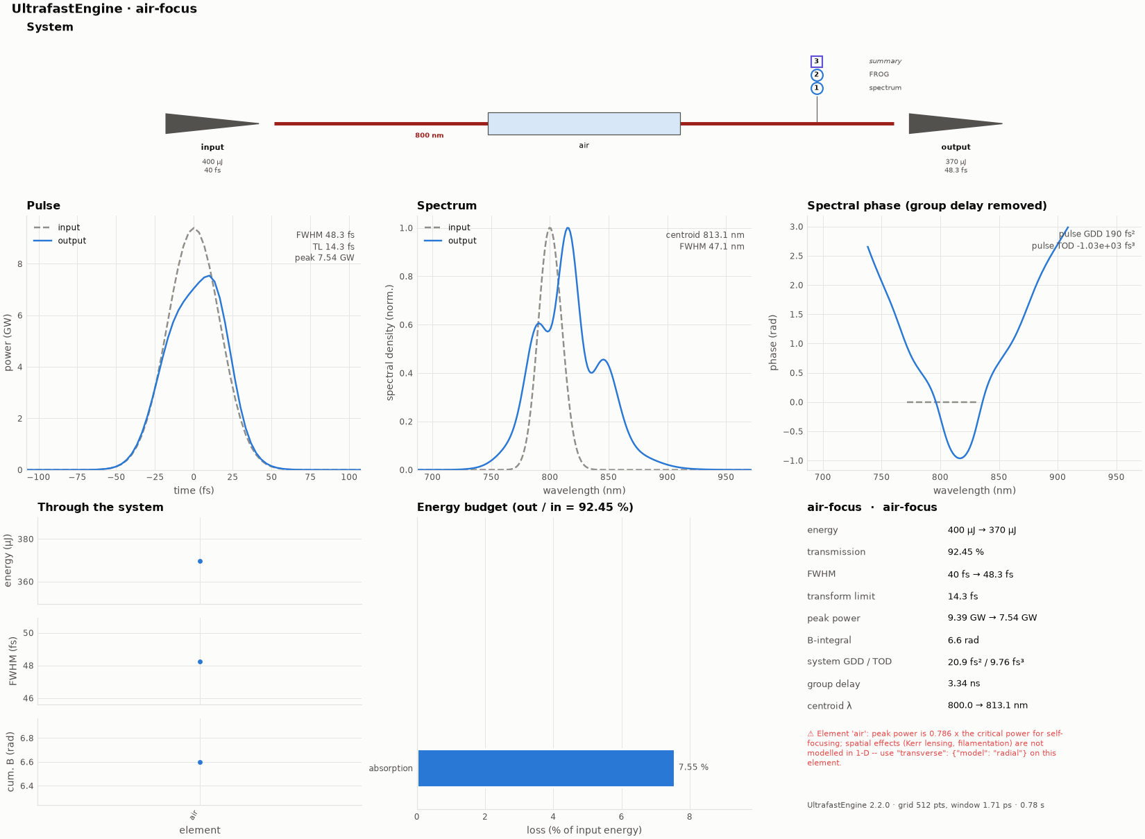
The overview figure of this example's run (python make_figures.py redraws it; the file is hero.png).

ultrafast run cell.ufs run.json -o results                        # ~2 s
ultrafast retrieve pcgpa results/result.npz -o retrieved           # FROG -> pulse (the frog instrument's trace)

What to look at:

• summary.json → elements[0].values: peakElectronDensityM3 (~1.9·10²² m⁻³) and peakIonizationFraction (~7·10⁻⁴).
• The spectrum broadens (B ≈ 6.6 rad) and its centroid moves to the red (815 nm): the delayed rotational response red-shifts the trailing part of the pulse more than the weak plasma blue-shifts the leading part.
• The FROG and its retrieval: retrieved/retrieval.json (G ≈ 10⁻⁵, FWHM 50.3 fs vs 51.3 fs simulated); retrieved/retrieved_spectrum.csv can be the input of another run ("pulse": {"shape": "spectrum", "spectrum": {"csv": "retrieved/retrieved_spectrum.csv"}, "energyJ": 3.7e-4}).

1-D caveat: the peak power is 0.8 of the critical power of air, and the engine warns that self-focusing is not modelled. For a real filament give the element "transverse": {"model": "radial", "points": 128, "radiusM": 1e-3, "equation": "uppe"} (much slower: minutes).

Try: "rotationalRaman": false on a custom air material, or "ionization": false, and compare the spectra. "ionization": {"frequencyResolved": false} applies the Drude index at the carrier only, as versions before this one did: the centroid moves to 813 nm and the energy loss drops from 8.8 % to 7.5 %, because the electrons born in the field also take their drift energy U_p in the frequency-resolved model (Ionisation).