30 -- Diffraction by an iris: four beam shapes, four distances¶

Four beams pass a 1 mm iris and are imaged at four distances. The beams are a Gaussian (w = 2 mm), a round flat-top (super-Gaussian of order 10, w = 1.5 mm), a uniform beam (a hard-edged tophat of radius 3 mm, a plane wave as far as the iris is concerned) and a square flat-top (half-width 1.5 mm). The round beams pass a round iris of radius a = 1 mm; the square beam passes a 2 x 2 mm square aperture. 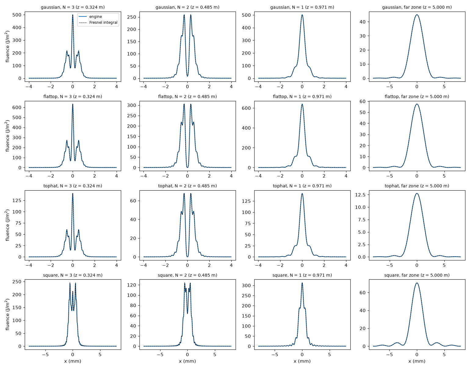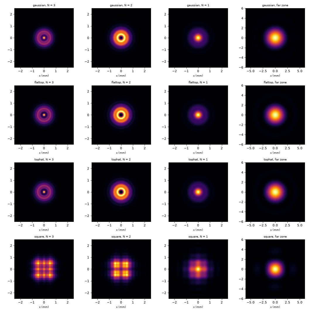The distances are where the Fresnel number N = a² / (λ z) of the opening is 3, 2 and 1, and the far zone at 5 m (N = 0.19). compare.py checks every pattern against the Fresnel diffraction integral. The step-by-step version is Tutorial 6: Diffraction by an iris.

cd docs/examples/Diffraction/iris-diffraction
for b in gaussian flattop tophat square; do ultrafast run $b.ufs run.json -o results-$b; done   # 2-5 s each
python compare.py            # engine vs Fresnel integral; writes diffraction-cuts.png, diffraction-images.png

Each system is a zero-length gap that sets the beam (transverse.initialProfile), the aperture, and free-space gaps to the four planes. Every element has the same grid, so the profile is handed on unchanged:

"transverse": { "model": "radial", "points": 1024, "radiusM": 12e-3, "absorbingBoundary": true,
                "initialProfile": { "kind": "tophat", "radiusM": 3e-3 } }          // or gaussian / flatTop; square: "geometry": "square"

• Radial grid, 1024 points over 12 mm (11.7 µm steps, 85 samples across the iris radius). The square case uses a cartesian grid, 512 x 512 over 24 mm (47 µm, 21 samples across the half-width), with "spectralSamples": 4: a 1 ps pulse needs only a few stored frequencies, and memory scales with them.
• absorbingBoundary: a hard edge sends light to large angles. Without the absorber that light reflects at the edge of a radial grid (and focuses back onto the axis) or wraps around a cartesian one. The absorbed energy is booked as grid boundary and reported as absorbedAtBoundaryFraction: 0.07 % at N = 3, 0.45 % at N = 1 and 3.9 % at 5 m for the uniform beam -- the outer Airy rings, which at 5 m lie beyond the 12 mm window (they are real light at angles above ~2 mrad).
• Linear gaps propagate only the profile at its stored frequencies (representation in summary.json says so), so each run takes a few seconds.

Expected output¶

python compare.py (fresh runs, Apple-silicon laptop). F(0) is the fluence on the axis (radial grids: the first sample, r = 11 µm); max err is the largest difference between the engine and the Fresnel integral over the pattern, as a fraction of its peak:

beam      at      z (m)      N  T iris    F(0) engine   F(0) Fresnel    max err
gaussian  n3     0.3236      3  0.3926          499.6          500.1      0.09%
gaussian  n2     0.4854      2  0.3926          7.976          7.949      0.03%
gaussian  n1     0.9709      1  0.3926          502.3          500.1      0.45%
gaussian  far    5.0000   0.19  0.3926          44.94          44.95      0.01%
flattop   n3     0.3236      3  0.4992          632.2          632.9      0.10%
flattop   n2     0.4854      2  0.4992        0.00482       0.001678      0.03%
flattop   n1     0.9709      1  0.4992          640.3            637      0.52%
flattop   far    5.0000   0.19  0.4992          57.48          57.49      0.01%
tophat    n3     0.3236      3  0.1108          140.4          140.5      0.05%
tophat    n2     0.4854      2  0.1108        0.001049      0.0003552      0.06%
tophat    n1     0.9709      1  0.1108          142.2          141.4      0.57%
tophat    far    5.0000   0.19  0.1108          12.76          12.76      0.04%
square    n3     0.3236      3  0.4945            212          213.8      1.30%
square    n2     0.4854      2  0.4945          63.55          63.81      0.75%
square    n1     0.9709      1  0.4945          313.4          313.3      0.25%
square    far    5.0000   0.19  0.4945          70.59          70.94      0.48%
largest difference over all patterns: 1.30 % of the peak

What to read from it:

• Fresnel zones. For the uniform beam the axis is bright, 4 x the incident fluence, at odd N (4 x 35.4 = 141.5 J/m²) and dark at N = 2: the iris then holds exactly two Fresnel zones, whose waves cancel on the axis (Born & Wolf, Principles of Optics, 8.8). The flat-top does the same. For the Gaussian the edge wave is weaker (the field at the edge is e^-0.25 of the centre), so the centre at N = 2 is dim, not dark.
• Transmission. The iris passes 1 − exp(−2a²/w²) = 39.35 % of the Gaussian (engine 39.26 %), (1/3)² = 11.11 % of the uniform beam (11.08 %), and 50.07 % / 50.25 % of the round / square flat-tops (49.92 % / 49.45 %). The grid cells on the edge transmit the fraction of their area inside the opening. That puts the edge in the right place between samples, but light diffracted beyond the grid's largest angle is lost, so the transmission converges from below, by about dx / 3a times the edge fluence (1.6 % for the square at 21 samples, 0.6 % at 1024 x 1024).
• The far zone is the Fraunhofer pattern: the Airy disc of the round iris, first dark ring at 0.61 λz/a = 3.14 mm, and the sinc² of the square, first zero at λz/2a = 2.58 mm along x.

Things to try¶

• Grids. Halve points (radial) or nx/ny (square) and run compare.py again: the errors grow. With fewer than 10 samples across the opening the engine warns that the aperture is under-resolved. Turn absorbingBoundary off and watch the far-zone pattern of the square pick up the light that wrapped around (about 19 % error on the axis).
• Near field. At N = 19 (z = 5 cm) the outermost Fresnel zone at the edge is λz/2a = 26 µm wide; the grid needs several samples across it (dx = 11.7 µm radial gives 2, the 47 µm cartesian grid less than 1): refine the grid before trusting the pattern there.
• A pinhole filter. Put a lens before the iris and the iris in its focal plane (the beam's Fourier plane) to clean a beam up, or replace the iris by a soft aperture ("softRadiusM", "order") to suppress the rings.
• Broadband light. Use a 20 fs pulse: every colour has its own Fresnel number, so the fine rings of the near field average out (Transverse: chromatic diffraction); keep the default 48 spectralSamples.